Bias-Variance Analysis of Local Classification
Methods
Julia Schiffner, Bernd Bischl and Claus Weihs
AbstractIn recent years an increasing amount of so called local classification meth-ods has been developed. Local approaches to classification are not new. Well-known examples are theknearest neighbors method and classification trees (e. g. CART). However, the term ‘local’ is usually used without further explanation of its partic-ular meaning, we neither know which properties local methods have nor for which types of classification problems they may be beneficial. In order to address these problems we conduct a benchmark study. Based on 26 artificial and real-world data sets selected local and global classification methods are analyzed in terms of the bias-variance decomposition of the misclassification rate. The results support our intuition that local methods exhibit lower bias compared to global counterparts. This reduction comes at the price of an only slightly increased variance such that the error rate in total may be improved.
1 Introduction
Lately the amount of literature on local approaches to classification is increasing. The probably best-known example is theknearest neighbors method. Many more lo-cal approaches have been developed, most of them can be considered lolo-calized ver-sions of standard classification techniques such as LDA, logistic regression, na¨ıve Bayes, SVMs, neural networks, boosting etc. The main idea of local classification methods is as follows: Since it is often difficult to find a single classification rule that is suitable for the whole population, rather concentrate on subsets of the pop-ulation and calculate several individual rules that are only valid for single subsets. Two questions immediately arise: What is the effect of this localization and in which situations are local methods especially appropriate? Many authors when proposing
Julia Schiffner·Bernd Bischl·Claus Weihs
Department of Statistics, TU Dortmund University, 44221 Dortmund, Germany, e-mail: [email protected]
a new local classification method just demonstrate superior performance over stan-dard methods on selected data sets. To our knowledge there are only few theoretical results regarding the performance of local methods and no extensive studies that compare several types of local methods across many data sets. A useful concept to gain deeper insight into the behavior of learning algorithms is the bias-variance decomposition of prediction error. It was originally introduced for quadratic loss functions, but generalizations to the misclassification rate have been developed. In a benchmark study on real-world and synthetic data we assess the bias-variance de-composition of the misclassification rate for different types of local methods as well as global methods. For a start in Sect. 2 a short introduction to local approaches to classification is given and different types of local methods are described. The bias-variance decomposition of the misclassification rate and its specific properties are explained in Sect. 3. The benchmark study and the results are presented in Sect. 4. Finally, in Sect. 5 a summary and an outlook to future work are given.
2 Local Approaches to Classification
Due to space limitations we can only give a short introduction. We do not go into details here, but rather point to references on certain topics. In classification it is assumed that each objectωin the populationΩ belongs to one and only one class
y=Y(ω)∈Y, withY denoting the set of class labels. Additionally, on each object
measurements x=X(ω)∈X are taken. Both,X andY, are assumed to be ran-dom variables. The aim is to find a classification rule or classifierD:X →Y that
based on the measurements predicts the class labels. The setX is usually called
predictor space and oftenX ⊂Rd. A local classifier is specialized on subsets of
the populationΩ. A local classification method induces one or more local classifiers
and aggregates them if necessary. According to which subsets of the population are addressed several types of local approaches can be distinguished:
Observation-Specific Methods For each object in the population an individual clas-sification rule is built based on the training observations near the trial pointx. The best-known example is kNN. But in principle every classification method can be localized this way, for example a localized form of LDA is described in Czogiel et al (2007). While for kNN locally constant functions are fitted to the data, in case of LLDA locally linear functions are used. A review paper concerned with observation-specific methods is Atkeson et al (1997).
Partitioning Methods These methods partition the predictor spaceX. Examples
are CART, mixture-based approaches like mixture discriminant analysis (MDA, Hastie and Tibshirani, 1996) and other multiple prototype methods like learning vector quantization (LVQ, Hastie et al, 2009). Strictly speaking kNN belongs to both groups because it generates a Voronoi tessellation ofX.
that are beyond the scope of this paper. Since in local classification model assump-tions need only be valid for subsets of the population instead of the whole population they are relaxed. For this reason localized methods exhibit more flexibility than their global counterparts and are expected to give good results in case of irregular class boundaries. Localization is only one way to obtain flexible classifiers. Other global ways are e. g. using polynomials of higher degrees and/or kernel methods.
3 Bias-Variance Decomposition of the Misclassification Rate
The bias-variance decomposition of prediction error was originally introduced for quadratic loss. The two main concerns when generalizing it beyond quadratic loss are finding reasonable definitions of bias and variance on the one hand and deriving the decomposition of prediction error on the other hand (e. g. James, 2003).
Definitions of Noise, Bias and Variance LetPX,Y denote the joint distribution ofX
andY and letP(Y=y|x)be the class posterior probabilities. In classification noise at a fixed trial pointxis the irreducible or Bayes error
Var(Y|x) =EYL01 Y,S(Y|x)|x=1−max not fixed. Bias and variance are defined as
bias(Yˆ|x) =L01 S(Y|x),S(Yˆ|x)
is usually called the main prediction andIis the indicator function. Bias measures the systematic deviation of the main prediction fromS(Y|x), whileVar(Yˆ|x) indi-cates the random variation of ˆY around the main prediction.S is an operator that reveals the systematic parts ofY and ˆY. The definitions given here are natural gen-eralizations of those in the quadratic case, i. e. if the quadratic loss is used instead ofL01they reduce to the standard definitions of noise, squared bias and variance.
EY,YˆL01(Y,Yˆ)|x=Var(Y|x) +bias(Yˆ|x) +Var(Yˆ|x)−2Var(Y|x)bias(Yˆ|x)
−2Var(Y|x)Var(Yˆ|x)−2bias(Yˆ|x)Var(Yˆ|x) +4Var(Y|x)bias(Yˆ|x)Var(Yˆ|x). (6)
In contrast to the quadratic case the decomposition additionally contains interac-tions. The negative interaction effect of bias and variance indicates that variance corrects the prediction in case of bias. If the number of classes is larger than two this correction does not occur for sure, but with a certain probability, which makes the decomposition even more complicated.
Systematic and Variance Effects In order to obtain a simpler decomposition James (2003) distinguishes between bias and variance as measures of systematic deviance and random variation on the one hand and the effects of bias and variance on the prediction error on the other hand. He defines systematic and variance effects as
SE(Y,Yˆ|x) =EYL01 Y,S(Yˆ|x)−L01 Y,S(Y|x)|x, (7)
VE(Y,Yˆ|x) =EY,YˆL01(Y,Yˆ)−L01 Y,S(Yˆ|x)|x. (8)
The systematic effect is the change in prediction error if instead of the Bayes pre-dictionS(Y|x)the main predictionS(Yˆ|x)is used. The variance effect measures the change in prediction error due to random variation of ˆY around the main predic-tion. WhileSE(Y,Yˆ|x)≥0 the variance effect for the reasons explained above can also take negative values. Under squared loss bias and variance coincide with their respective effects. Generally, an estimator with zero bias also has zero systematic effect and an estimator with zero variance has zero variance effect. With system-atic and variance effects an additive decomposition of the misclassification rate is obtained as follows
EY,Yˆ
L01(Y,Yˆ)|x
=Var(Y|x) +SE(Y,Yˆ|x) +VE(Y,Yˆ|x). (9)
4 Benchmark Study
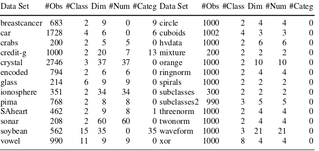
Table 1 Characteristics of the 26 data sets used in the benchmark study: Number of observations, number of classes, dimensionality, number of numeric and number of categorical predictors
Data Set #Obs #Class Dim #Num #Categ Data Set #Obs #Class Dim #Num #Categ
breastcancer 683 2 9 0 9 circle 1000 2 4 4 0
car 1728 4 6 0 6 cuboids 1002 4 3 3 0
crabs 200 2 5 5 0 hvdata 1000 2 6 6 0
credit-g 1000 2 20 7 13 mixture 200 2 2 2 0
crystal 2746 3 37 37 0 orange 1000 2 10 10 0
encoded 794 2 6 6 0 ringnorm 1000 2 4 4 0
glass 214 6 9 9 0 spirals 1000 2 2 2 0
ionosphere 351 2 34 34 0 subclasses 300 2 2 2 0
pima 768 2 8 8 0 subclasses2 990 3 5 5 0
SAheart 462 2 9 8 1 threenorm 1000 2 4 4 0
sonar 208 2 60 60 0 twonorm 1000 2 4 4 0
soybean 562 15 35 0 35 waveform 1000 3 21 21 0
vowel 990 11 9 9 0 xor 1000 8 4 4 0
local methods, we would like to know if there are differences between local methods and global approaches of similar flexibility.
Data Sets We consider 26 data sets, both artificial and real-world data. Most data sets are taken from the UCI repository (Frank and Asuncion, 2010) and the mlbench R-package (Leisch and Dimitriadou, 2010). The threenorm, twonorm and waveform data were used in Breiman (1996). The crystal and encoded data sets are described in more detail in Szepannek et al (2008), the mixture data are taken from Bishop (2006). The hvdata set is an artificial data set described in Hand and Vinciotti (2003). The orange and South-African-heart-disease (SAheart) data are taken from Hastie et al (2009) and the crabs data are available in the MASS R-package (Venables and Ripley, 2002). In Table 1 a survey of the data sets used in the study is given. On the left hand the real-world and on the right hand the artificial data sets are shown. The crabs and wine data sets as well as the hvdata and twonorm data sets pose relatively easy problems since the decision boundary is linear. The circle, orange, ringnorm, subclasses and threenorm data sets are quadratic and the xor and subclasses2 data sets are more complex classification problems.
Classification Methods We consider ten classification methods, three global and seven local methods.
• Global methods: We apply two linear methods, LDA and multinomial regression (MNR), and as a more flexible method a SVM with polynomial kernel (poly SVM). The degree of the polynomial is tuned in the range of 1 to 3.
• Partitioning methods: We consider CART, learning vector quantization (LVQ1) and mixture discriminant analysis (MDA, Hastie and Tibshirani, 1996).
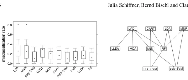
misclassification r
Fig. 1 Left: Boxplot of the error rates on the 26 data sets. Right: Consensus ranking of the classi-fication methods
• Moreover, we consider random forests (RF), which can be regarded as local clas-sification method in conjunction with an ensemble method. Since several classi-fication trees are combined RF normally exhibits lower variance than CART.
Measuring Noise, Bias and Variance In case of artificial data the noise level is usu-ally known. When dealing with real-world data noise can be estimated by means of a consistent classifier. We follow the proposition of James (2003) and employ the 3NN method where the neighbors are weighted by a Gaussian kernel. In order to calculate bias and variance we need to estimate the distribution of ˆY. For this pur-pose we use a nested resampling strategy. In the outer loop we employ subsampling (4/5 splits with 100 repetitions). The subsample is used for training while based on the remaining data error, bias, variance and their effects are estimated. In the inner loop we use 5-fold cross-validation for parameter tuning which is required for all employed classification methods except LDA and MNR. A more detailed descrip-tion of how bias, variance etc. can be estimated can be found in James (2003). All calculations were carried out in R 2.11.1 (R Development Core Team, 2009) using the mlr R-package (Bischl, 2010).
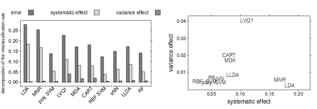
decomposition of the misclassification r
Fig. 2 Left: Error rates, systematic and variance effects averaged over the 26 data sets. Right: Variance effect versus systematic effect
and polynomial SVM show best performance. Moreover, there are no methods that beat LLDA and MDA. Both linear methods and LVQ1 exhibit highest error rates. Next, in order to explain the differences in error rates we consider the bias-variance decomposition. Fig. 2 shows the average misclassification rates as well as system-atic and variance effects over all 26 data sets. For all classification methods the systematic effects are considerably larger than the variance effects. Differences in error rates are mainly caused by changes in systematic effect. Both methods with lowest error rates, polynomial and RBF SVMs, exhibit the smallest systematic ef-fects. Their variance effects are hardly larger than that of LDA which is minimal under all classification methods. The localized versions of LDA, LLDA and MDA, both exhibit considerably lower systematic effects, but only slightly increased vari-ance effects. LVQ1 and as expected CART exhibit the largest varivari-ance effects. Com-pared to CART random forests (RF) shows a smaller average variance effect, but as well a smaller systematic effect. In order to visualize which classification methods show a similar behavior with respect to the bias-variance decomposition we plot the variance effect against the systematic effect. We can recognize two clusters, one formed by the linear methods LDA and MNR, the other one formed by highly flex-ible methodskNN, RF as well as RBF and polynomial SVM. Neither global and local methods nor the different types of local methods we mentioned in Sect. 2 can be distinguished based on this plot. The reason may be that the bias-variance de-composition only reflects the degree of flexibility of classification methods and that the way how it is obtained, by localization or otherwise, is not relevant.
5 Summary and Outlook
system-atic effect than global counterparts. Contrary to our assumptions most local methods under consideration, except LVQ1 and CART, only have a slightly increased vari-ance effect, the main contributors to prediction error are noise or systematic effect. In terms of the bias-variance decomposition neither global and local methods nor the different types of local methods could be distinguished. In the future we would like to apply more classification methods. Some types mentioned in Sect.2 like mul-ticlass to binary have not been included yet. Moreover, we plan to relate the results to characteristics of different types of local classification methods. All conclusions were drawn based on averages over the 26 data sets in the study, differences between distinct data sets are not taken into account. In order to gain deeper insight and to get hints in what situation which method will probably perform well it would be useful to relate the results to characteristics of the data sets.
References
Allwein EL, Shapire RE, Singer Y (2000) Reducing multiclass to binary: A unifying approach for margin classifiers. Journal of Machine Learning Research 1:113–141
Atkeson CG, Moore AW, Schaal S (1997) Locally weighted learning. Artificial Intelligence Review 11(1-5):11–73
Bischl B (2010) mlr: Machine learning in R. URL http://mlr.r-forge.r-project.org Bishop CM (2006) Pattern Recognition and Machine Learning. Springer, New York
Breiman L (1996) Bias, variance, and arcing classifiers. Tech. Rep. 460, Statistics Department, University of California at Berkeley, Berkeley, CA, URL www.stat.berkeley.edu
Czogiel I, Luebke K, Zentgraf M, Weihs C (2007) Localized linear discriminant analysis. In: Decker R, Lenz HJ (eds) Advances in Data Analysis, Springer, Berlin Heidelberg, Studies in Classification, Data Analysis, and Knowledge Organization, vol 33, pp 133–140
Eugster MJA, Hothorn T, Leisch F (2008) Exploratory and inferential analysis of benchmark exper-iments. Tech. Rep. 30, Institut f¨ur Statistik, Ludwig-Maximilians-Universit¨at M¨unchen, Ger-many, URL http://epub.ub.uni-muenchen.de/4134/
Frank A, Asuncion A (2010) UCI machine learning repository. University of California, Irvine, School of Information and Computer Sciences, URL http://archive.ics.uci.edu/ml
Hand DJ, Vinciotti V (2003) Local versus global models for classification problems: Fitting models where it matters. The American Statistician 57(2):124–131
Hastie T, Tibshirani R (1996) Discriminant analysis by Gaussian mixtures. Journal of the Royal Statistical Society B 58(1):155–176
Hastie T, Tibshirani R, Friedman J (2009) The Elements of Statistical Learning: Data Mining, Inference, and Prediction, 2nd edn. Springer, New York
James GM (2003) Variance and bias for general loss functions. Machine Learning 51(2):115–135 Leisch F, Dimitriadou E (2010) mlbench: Machine learning benchmark problems. R package
ver-sion 2.0-0
R Development Core Team (2009) R: A Language and Environment for Statistical Computing. R Foundation for Statistical Computing, Vienna, Austria, URL http://www.R-project.org Szepannek G, Schiffner J, Wilson J, Weihs C (2008) Local modelling in classification. In: Perner
P (ed) Advances in Data Mining. Medical Applications, E-Commerce, Marketing, and Theo-retical Aspects, Springer, Berlin Heidelberg, LNCS, vol 5077, pp 153–164