Non-published Research Reports
1-1-2009
Nominal Analysis of "Variance"
David J. WeissCalifornia State University - Los Angeles
Follow this and additional works at:htp://research.create.usc.edu/nonpublished_reports
his Article is brought to you for free and open access by CREATE Research Archive. It has been accepted for inclusion in Non-published Research Reports by an authorized administrator of CREATE Research Archive.
Recommended Citation
Weiss, David J., "Nominal Analysis of "Variance"" (2009).Non-published Research Reports.Paper 36.
Running head: NOMINAL ANALYSIS
Nominal Analysis of “Variance”
David J. Weiss
Abstract
Nominal responses are the natural way for people to report actions or opinions. Because
nominal responses do not generate numerical data, they have been under-utilized in
behavioral research. On those occasions where nominal responses are elicited, the
responses are customarily aggregated over people or trials so that large-sample statistics
can be employed. A new analysis is proposed that directly associates differences among
responses with particular sources in factorial designs. A pair of nominal responses either
matches or does not; when responses do not match, they vary. That analog to variance is
incorporated in the Nominal Analysis of “Variance” (Nanova) procedure, wherein the
proportion of non-matches associated with a source plays the same role as sum of squares
does in analysis of variance. The Nanova table has the same structure as an analysis of
variance table. The significance levels of the N-ratios formed by comparing proportions
are determined by resampling. Fictitious behavioral examples featuring independent
groups and repeated measures designs are presented. A WINDOWS program for the
analysis is available.
Nominal Analysis of “Variance”
A nominal response is a verbal label. Asking for a nominal response is often the
natural way to elicit an opinion. The mechanic making a diagnosis, the potential
purchaser choosing a brand, and the possibly prejudiced person expressing a preference
are likely to be thinking of a label as they consider their response. Actions that people
intend or report having executed are also expressed nominally. In survey research,
nominal responses arise frequently.
Experimentalists, on the other hand, generally try to avoid tasks that generate
nominal data. In the laboratory, a familiar task may be altered so that numerical data can
be provided. For example, suppose an investigator wishes to study how physicians
evaluate hypothetical patients whose symptoms are varied systematically. So that the
judgments can be expressed numerically, the physician might be asked to predict how
many months the patient can be expected to survive, or the probability that the patient
will survive until a particular point in time. Although the latter judgments are medically
pertinent, they are more complex than merely identifying the disease and perhaps
recommending a regimen, tasks that arise routinely in medical practice.
To be sure, experimenters have been trained to gather numerical data for good
reasons. Numerical data provide more information and more analytic power than nominal
data. Quantitative theories are more interesting than qualitative ones, and it seems
obvious that numerical data are needed to test a quantitative theory. Simply reporting
nominal responses may pose a challenge; how are they to be aggregated? Can nominal
Perhaps no single writer has had more influence on the data-gathering proclivities
of behavioral researchers than S. S. Stevens (1946, 1951). His discussions of the
constraints placed on statistical operations by the scale properties of the responses,
although vigorously challenged (e.g., Anderson, 1961; Lord, 1953), still lead
experimentalists largely to restrict nominal data to the demographics section of their
reports. Even if a researcher were willing to ignore Stevens’s proscription, nominal data
do not seem suitable for sophisticated experimental work. The elegant factorial designs to
which experimenters apply analysis of variance require numerical data. Yet there are
many tasks for which nominal responses are the most appropriate, and requiring
participants to use other modes smacks of the carpenter who pounds in screws because
the only available tool is a hammer.
In this paper, I present a method for analyzing nominal responses collected using
factorial designs. The goal is to allow the analytic power afforded by factorial designs to
be extended to studies in which nominal responses are the natural way to express a
person’s actions or judgments. That is, I echo Keppel’s (1991) assertion that the intimate
connection between design and analysis is conducive to the conceptualization of incisive
studies.
Of course, nominal responses do not exhibit variance in the usual sense, since
there is no metric that that can support measures of distance. One cannot say by how
much two nominal responses differ. Still, it is possible to invoke the concept of disparity
between responses, in that two responses either match or do not match. The proposed
by the experimental design. This partitioning corresponds to the orthogonal partitioning
of sums of squares characteristic of analysis of variance.
Nominal analysis
The fundamental statistic in the proposed nominal analysis of variance (Nanova)
is the proportion of non-matches, which compares obtained and potential matches
associated with a source. The algebraic expression for the proportion is (Potential –
Obtained)/Potential. The number of potential matches associated with each of the sources
is inherent in the design structure, while the number of obtained matches is an empirical
outcome. Every potential match is assigned to a unique source; this is the sense in which
the partitioning is orthogonal.
The rationale for placing non-matches (the complement of obtained matches) in
the numerator of the proportion is that when responses to the various levels of a factor are
the same (the nominal version of the usual null hypothesis), that factor does not affect the
response. Accordingly, the obtained proportion of non-matches ought to be small if that
null hypothesis is true. Proportions of non-matches range between 0 and 1, and are
analogous to effect sizes.
Significance questions are addressed in the Nanova table. The proportions of
non-matches play the role of mean squares in analysis of variance, in that they are combined
in a ratio format to yield the test statistic, the N-ratio. The N-ratio compares the
proportion of non-matches for a substantive source to the proportion of non-matches for
the error term associated with that source. The selection of the error term for a source
follows the traditional rules of analysis of variance. It should be noted that, although
proportions as presented by Dyke and Patterson (1952). The data they analyze are
proportions, whereas the data for Nanova are individual responses.
The expected value of an N-ratio under the usual null hypothesis of no differences
is 1, just as for an F-ratio. Because there are no underlying distributional assumptions,
significance tests on N-ratios are carried out using a resampling procedure (Edgington &
Onghena, 2007). The observed scores are randomly permuted without replacement
(Rodgers, 2000) a “large” number of times; I use 100,000 as the default large number.
After each permutation, N-ratios for each substantive source are calculated. The
proportion of times the N-ratio derived from permuted data exceeds the N-ratio from the
original data is an estimate of the probability of obtaining an N-ratio at least that large
given the null hypothesis is true, thereby corresponding to a p value in analysis of
variance. The logic is that the resampled data were not truly generated by the factors, so
any patterns emerging in the proportions of non-matches are fortuitous.
Antecedents
A definition of variance for nominal data was first proposed by Gini (1939), who
suggested examining all n2 pairs of ordered responses in a set. A pair that matches
generates a difference of 0, and a pair that does not match generates a difference of 1.
Gini defined the sum of squares for the set of n responses to be the sum over all pairs of
the squared differences divided by 1/2n. Gini’s definition is related to Nanova’s
proportion of non-matches. Because Gini cleverly chose 0 and 1 as the seemingly
arbitrary constants for describing matches and non-matches (02 = 0 and 12 = 1), Gini’s
Light and Margolin (1971) built a true analysis of variance procedure for
categorical data on Gini’s definition, partitioning the total sum of squares into between
and within terms. They compared their F-tests to equivalent chi-square contingency
statistics and found the former to be more powerful under some circumstances. Onukogu
(1985) also constructed an analysis of variance for nominal data, but his sums of squares
incorporate a slightly different divisor than those of Gini and of Light and Margolin. Both
of these published analyses were illustrated with a large data set.
Nanova’s key quantities, the proportions of non-matches, are members of the
same family as Gini’s sum of squares, but do not yield F-ratios. The Light and Margolin
(1971) and Onukogu (1985) procedures are presented for designs with only one
substantive factor. Nanova is more general, allowing for multifactor designs and
providing estimates of main effects and interactions.
Multiway contingency analyses (Goodman, 1971; Shaffer, 1973) also apply
factorial decomposition to nominal responses and may be seen as competitors to Nanova.
Other competitors include loglinear analysis (Agresti, 1990) and multinomial logit
analysis (Grizzle, 1971; Haberman, 1982; McFadden, 1974). In these multifactor
generalizations of traditional chi-square tests of independence, all of the classifications
have equivalent status. On the other hand, Nanova distinguishes between its dependent
variable and its independent variable(s). From the expermentalist’s standpoint, this
distinction is meaningful, which is why analysis of variance continues to thrive despite
Cohen’s (1968) demonstration that equivalent insights can be extracted from multiple
regression.
A multinomial model is a plausible choice for nominal data (Bock, 1975). A
response is viewed as a random variable that assumes an integer value j with probability
pj. Responses are presumed to be independent. The binomial model is a special case of
the multinomial model used for dichotomous responses, where j takes on one of two
possible values. For categorical responses, j takes on a range of values equal to the
number of categories. The pj’s are estimated with response proportions.
However, the Nanova analysis is not restricted to categorization tasks. The
computations are the same whether responses were emitted freely or elicited with
multiple-choice items. While the usual multinomial assumption of a fixed set of
probabilities is appropriate for a categorization task, it seems less applicable to free
responding. Removing the constraints threatens to yield data matrices featuring unique
responses or empty cells, both of which pose problems of estimability for generalized
linear models (Fienberg, 2000). Instead, following Smith (1989), I follow a more general
course by viewing the multinomial population as being sampled from an unknown
distribution.
Specific multinomial models, such as the multinomial logit, propose specific error
distributions for the response. In developing Nanova, I preferred to avoid specifying an
error distribution because any such proposal might be incorrect. Use of the randomization
test for assessing significance obviates the need to elaborate the sampling distribution of
the new N-ratio statistic. Because the distributional assumptions are bypassed, the use of
Nanova does not require consideration of asymptotic properties. Accordingly, large
samples are not required, although large samples might be expected to convey the usual
Examples
In these examples, I use fictional experiments and artificial data to illustrate the
kinds of studies for which Nanova might be suitable and how the matches are assigned to
sources. In the illustrations, I use single letters as the responses to simplify the
presentation; but the responses could as well be words spoken or written by respondents,
or they might be verbal descriptions of actions. I first show a one-way, independent
groups design and compare the analysis with a conventional contingency table analysis
using a chi-square test. Then I show two repeated measures analyses using the same
design, with data constructed to show first a stimulus effect and then a subject effect.
These results serve as a check on the validity of Nanova, in that the analysis captures the
different effects I built into the data. The third example, a two–factor independent groups
design, illustrates how Nanova handles interaction. Additional examples, including one
featuring a mixed design with a nested subjects factor, are posted at
http://www.davidjweiss.com/NANOVA.htm.
Although one can count matches manually, the process becomes mind-boggling
as the designs get larger and/or more complex. I recommend use of the NANOVA
computer program1, which also handles the resampling. 100,000 repetitions yielded
stable p-values for all of the examples presented here. None of the analyses took more
than 1 minute on a Core 2, 2.0 GHz computer. The program reports degrees of freedom
in the Nanova table to maintain correspondence with analysis of variance, but df are not
involved in the computations.
The Nanova tables in the examples highlight the most important practical
manner that is familiar to experimentalists. This clarity is especially valuable for designs
with multiple factors. The results look like analysis of variance tables, and the
contributions of the factors are interpreted in much the same way. In contrast, estimating
say, the multinomial logit model (Chen and Kuo, 2001), can get quite complicated2.
Example 1: Independent groups design
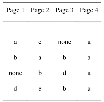
In the experiment reported in Table 1, 16 buyers saw one of four web pages and
then purchased either product a, b, c, d, e, or nothing (after Fasolo, McClelland, & Lange,
2005). This is a one-way, independent groups design with four scores per cell. The null
hypothesis is that what was purchased does not depend upon which page the buyer saw;
the alternative hypothesis is that the page does influence the purchase. Of course, with
nominal data, hypotheses are never directional. The hypothesis is tested by asking
whether the proportion of non-matches between columns is equal to the proportion of
non-matches within columns.
---
Insert Table 1 here
---
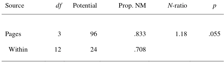
The overall number of potential matches is always the combination of the number
of responses taken two at a time. Over this set of 16 responses, there are 120 potential
matches (16C2). Twenty-three matches occurred. The potential and obtained matches are
partitioned according to the factorial structure. If we consider the “between-groups”
matches, counted over different pages, there are 96 potential (4•12 + 4•8 + 4•4), of which
16 occurred3. So there are 80 non-matches, yielding a proportion of non-matches of 80/96
matches (4•4C2), of which 7 occurred4. There are 17 non-matches, yielding a proportion
of non-matches of 17/24 = .708. The obtained N-ratio is formed by comparing the
proportions of non-matches for sources as though they were mean squares in analysis of
variance. Here, N = .833/.706 = 1.18.
---
Insert Table 2 here
---
In the resampling analysis, the proportion of times the N-ratio from permuted
data exceeded the N-ratio obtained from the original data (1.18) was .055, corresponding
to a p value of .055 in analysis of variance. According to standard null hypothesis testing
logic, these results are consistent with the null hypothesis at the .05 level of significance;
the page does not affect the purchase.
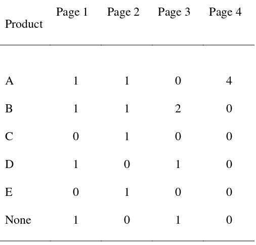
The usual way in which data suitable for a one-way, independent groups Nanova
are analyzed is with a chi-square test of independence. In Table 3, the data from Table 1
are displayed in a contingency table, wherein the entries are the number of people who
bought a particular product after seeing a particular page. The null hypothesis for the
chi-squaretest of independence is logically equivalent to that of one-way Nanova. Table 3
appears rather sparse, because this mode of presentation is poorly suited to the structure
of the data set in that some products were never chosen in response to particular pages.
Consequently, the data may be inappropriate for a standard chi-square test of
independence (a topic debated intensely 60 years ago, e.g., Lewis & Burke, 1949).
Ignoring that concern, I calculated the chi-square observed as 18.0. With 15 df, the
---
Insert Table 3 here
---
Example 2: Repeated measures design
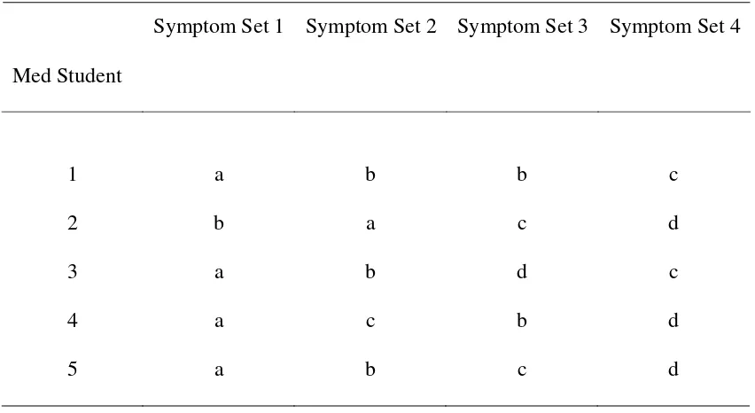
In Tables 4 and 6, the data are clinical diagnoses made by medical students. The
responses are unconstrained, in that no set of possible diseases from which to choose was
provided. The students named the disease (here, signified by the letters a, b, c, or d) they
attributed to a patient who had the designated set of symptoms. This is a 4 (Symptom sets)
x 5 (Medical students) repeated-measures design. Whereas in typical studies that examine
diagnosis, the outcome measure is likely to be accuracy, here we explore the process
question of how variation in the symptoms induces variation in the diagnoses. The data in
Table 4 were constructed to show a “symptom” effect. That is, the medical students
generally agreed on the diseases suggested by the symptom sets.
---
Insert Table 4 here
---
There are 190 (20C2) potential matches generated by the 4x5 design; 41 occurred.
There are 30 (5•4C2) potential matches across rows, of which 1 occurred. Within columns,
there are 40 (4•5C2) potential matches; 15 occurred. The “error term”, the usual subject x
treatment interaction in repeated-measures analysis of variance, looks at non-matches not
associated with either rows or columns. There are 120 (190 – 30 – 40) potential matches
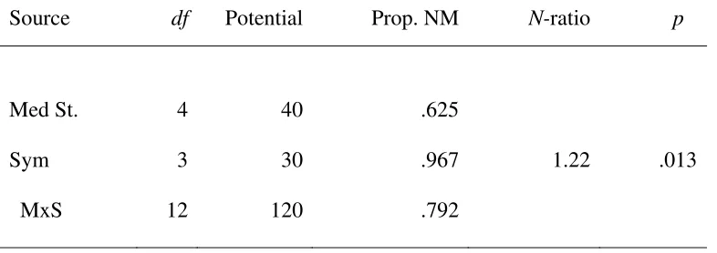
contributing to that interaction; 25 occurred. As shown in Table 5, the N-ratio of 1.22
---
Insert Table 5 here
---
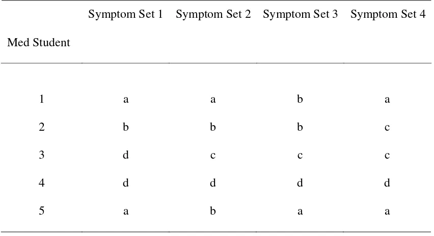
In contrast, the data in Table 6 were constructed to show a “subject” effect. Each
medical student tends to give an idiosyncratic diagnosis without much regard for the
symptoms.
---
Insert Table 6 here
---
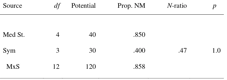
This time, the N-ratio for Symptoms is small, considerably less than the expected
value of 1 (perhaps I went overboard in constructing data with no symptom effect). The
p-value of 1 may have arisen because the program rounds proportions greater than .99995
up to 1.
---
Insert Table 7 here
---
Thus, the NANOVA analyses in both Tables 5 and 7 are detecting what was built
into the data. In Table 5, where subjects interpret the differential symptom information in
much the same way, the N-ratio for symptoms is “large”. In Table 7, subjects tend to
respond the same way regardless of the symptoms, and correspondingly the N-ratio for
symptoms is “small”. This difference is perhaps the strongest evidence for the promise of
the proposed technique, in that the N-ratio is responsive to effects in the data.
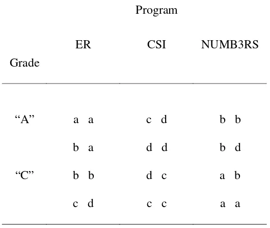
Table 8 illustrates how matches are counted for a two-factor (3 Programs x 2
Grades), independent groups design with 4 scores per cell. In this study, sixth-grade
children who had earned either “A” or “C” grades in science last year were assigned to
write a synopsis of a specific television program they were asked to watch. The
programs, all featuring scientists of a sort, were shown at 10 PM and not normally seen
by these young viewers. One week later, all of the students were asked to list three
careers they were considering. The children’s first responses were examined to see
whether the program assignment differentially influenced career consideration, and
whether this effect depended on the child’s previous success in science. In this case, the
responses are careers.
---
Insert Table 8 here
---
For the within-cells proportion that serves as the error term, we count the matches
within each of the 6 cells. There are 4C2 = 6 potential matches within each cell, resulting
from the pairing of each response with every other response in the cell, yielding 36
potential matches.
For the substantive sources, we count matches between responses for specified
pairs of cells. For the P main effect, we count matches among cells across rows. Each
response in cell P1G1 is compared to each response in cell P2G1 (no matches). Similar
comparisons are made for cell P1G1 with cell P3G1 (3 matches), cell P2G1 with cell P3G1
(3 matches), cell P1G2 with cell P2G2 (4 matches), cell P1G2 with cell P3G2 (2 matches),
The G main effect results from counting matches among cells down columns.
Responses in cell P1G1 are compared with those in cell P1G2 (2 matches), cell P2G1 with
cell P2G2 (6 matches), and cell P3G1 with cell P3G2 (3 matches).
The null hypothesis for Nanova interaction is that the response distribution across
the levels of one factor does not differ over the various levels of the other factor. The test
of interaction checks for matches among cells that are not in the same row or column. To
examine the PG interaction in the data presented in Table 8, we compare the four
responses in cell P1G1 with those in cell P2G2 (no matches). We continue by comparing
cell P1G1 with cell P3G2 (10 matches), cell P2G1 with cell P1G2 (4 matches), cell P2G1
with cell P3G2 (no matches), cell P3G1 with cell P1G2 (7 matches), and cell P3G1 with cell
P2G2 (1 match).
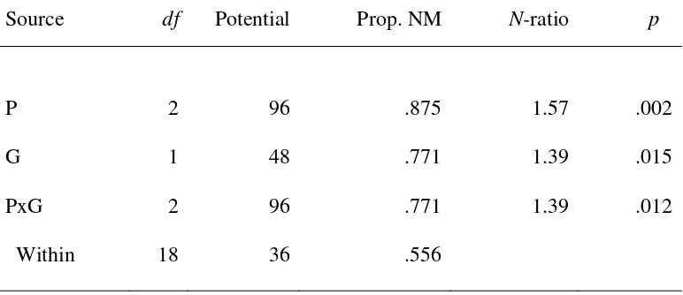
Each of the 276 (24C2) potential matches generated by the design is associated
with exactly one of the sources. Results are shown in Table 9. Programs and Grades both
affected career choice, but the significant interaction tells us that these factors did not
operate independently.
---
Insert Table 9 here
---
Preprocessing the data
Carrying out Nanova requires decisions about whether each pair of responses
matches. The simplistic interpretation of matching is that the responses must be identical.
When constrained response options are offered, that determination is easy to accomplish
researcher may have to judge whether a pair of non-identical responses ought to be
counted as a match.
Declaring linguistic equivalents as matches seems innocuous. If two different
words are true synonyms, the analyst may enter one of them both times. The use of
different languages by respondents also justifies substitution. A more delicate judgment is
required when one response is effectively a subset of another. For example, during a
study examining the effectiveness of automobile advertising, the participant may be
asked to name the kind of car she wants to buy. If the response is “Camry”, is that a
match with “Toyota”? “Camry” is certainly closer to “Toyota” than it is to “Ford.” The
researcher will have to make a decision. Such fuzzy matches were explored by Oden
(1977), who asked people to judge, for example, the extent to which a bat is a bird. It may
be feasible to devise a generalization of Nanova that incorporates degree of closeness,
where 0 means no match, 1 means identical, and intermediate values capture the extent to
which non-identical responses overlap in meaning.
Power considerations
It seems obvious that nominal data afford less power than numerical data, but how
much less? Power will be affected by the variety of responses the participant chooses. If
only a few alternatives are exercised, there will be many matches. Matches associated
with the error term increase power, while matches associated with substantive sources
decrease power. In some circumstances, the number of alternatives used will depend
upon the participant’s verbal habits or base rates for particular response options.
Because there is no assumption made about the underlying distribution of
two exercises to examine how power in the Nanova context compares to power in
analysis of variance.
When the data are homogeneous, one would expect power to increase with the
size of the data set. To test this prediction, I increased the size of the data set in Table 1
by duplicating the responses repeatedly. With one duplication (df = 3, 28; potential
matches = 384, 112), the N-ratio increased to 1.37. With two duplications (df = 3, 44;
potential matches = 864, 264), N was 1.44. With three duplications (df = 3, 60; potential
matches = 1536, 480), N was 1.47. The latter three N-ratios all yielded a p-value of <.001.
In this exercise, the power gain from replication was achieved entirely from increases in
the proportion of non-matches in the within term, because with perfectly replicated
responses the proportion of non-matches associated with pages remains constant.
The other slant on power compared numerical responses to nominal responses.
One would expect numerical data to afford more power. I computed an ordinary F-ratio
after replacing the letters in Table 1 with their ordinal positions in the alphabet, and the
“none” responses with zeros. If the study had been a real one, the numbers might
represent time spent looking at the page or amount of money spent after viewing it. The
comparison is via the p-values. To my surprise, the p-value was much higher (.564),
suggesting less power for the numerical data. The resolution is that the advantage of
numerical responses is that while they are inherently more sensitive to fine distinctions
respondents may make, my substitution was linked to distinctions that had already been
made using nominal responses. So notwithstanding the inappropriateness of this mode of
comparison, the result does suggest that Nanova is not an inherently weak test.
An intriguing methodological possibility offered by the Nanova procedure is
parallel assessment, by which I mean studies that collect numerical and behavioral
responses to the same stimuli. This is really an old idea, going back at least to a classic
study in which LaPiere (1934) compared racial attitudes expressed by, and actions taken
by, Southern innkeepers. One might examine how medical warnings varying in length
and intensity affect the patient emotionally, and at the same time see whether the same
factors inspire behavioral change. Studies of training might look at how instructional
innovations affect both knowledge and choice of action. Nominal responding is the
natural mode for expressing a choice, and the study of what underlies choices can
perhaps best be accomplished with the analytic power of factorial designs.
Nominal data are inherently less informative than quantitative data. Nominal data
cannot be averaged, cannot be graphed, and do not convey information about the
magnitude of differences. Because averaging is a meaningless operation, it is not clear
how to deal with missing data or inequality of cell sizes. However, nominal responses are
the natural mode for capturing actions, and a science of behavior ought to be able to
make use of them. Despite Stevens’s negative view, likely based on his pro-physics,
anti-psychology biases (Matheson, 2006), nominal data can provide valuable information in
Author Note
David J. Weiss, Department of Psychology, California State University, Los
Angeles.
This research was supported by the United States Department of Homeland
Security through the Center for Risk and Economic Analysis of Terrorism Events
(CREATE) under grant number 2007-ST-061-000001. However, any opinions, findings,
and conclusions or recommendations in this document are those of the author and do not
necessarily reflect views of the United States Department of Homeland Security. I am
grateful to Julia Pounds for suggesting the Nanova acronym and to Richard John, Jorge
Mendoza, and Rick Thomas for valuable comments regarding the manuscript.
Correspondence regarding this article, including requests for reprints, should be
sent to David J. Weiss, 609 Colonial Circle, Fullerton CA. 92835 United States. Email:
Footnotes
1. The NANOVA computer program is available for free download from
www.davidjweiss.com/NANOVA.htm. The WINDOWS program handles designs with
as many as four factors, including subjects or replicates.
2. Admittedly, the complexity, as well as the beauty, of an analysis is in the eye of the
beholder.
3. The “a” in the first column matches the “a” in the second column and each of the four
“a”s in the fourth column (running total of 5 matches). The “a” in the second column also
matches the four “a”s in the fourth column (running total of 9 matches). The “b” in the
second column matches the “b” in the second column and each of the two “b”s in the
third column (running total of 12 matches). The “b” in the second column also matches
the two “b”s in the third column (running total of 14 matches). There is one “none”
match (first and third column, running total of 15 matches) and one “d” match (first and
third column, final total of 16 matches).
4. The first and second columns have no matches. The “b”s in the third column match
(running total of 1 match). In the fourth column, the first “a” matches the second, third
and fourth “a”s (running total 4 matches), the second “a” matches the third and fourth
“a”s (running total 6 matches), and the third “a” matches the fourth “a” (final total of 7
References
Agresti, A. (1990). Categorical data analysis. New York: Wiley-Interscience.
Anderson, N. H. (1961). Scales and statistics: Parametric and nonparametric.
PsychologicalBulletin, 58, 305-316.
Bock, R. D. (1975). Multivariate statistical methods in behavioral research. New York:
McGraw-Hill.
Chen, Z., & Kuo, L. (2001). A note on the estimation of the multinomial logit model with
random effects. The American Statistician, 55, 89-95.
Cohen, J. (1968). Multiple regression as a general data-analytic system. Psychological
Bulletin, 70, 426-443.
Dyke, G. V., & Patterson, H. D. (1952). Analysis of factorial arrangements when the data
are proportions. Biometrics, 8, 1-12.
Edgington, E. S., & Onghena, P. (2007). Randomization tests (4th ed.). Boca Raton, FL:
Chapman & Hall/CRC.
Fasolo, B., McClelland, G. H., & Lange, K. (2005). The effect of site design and
interattribute correlations on interactive web-based decisions. In C. P. Haugtvedt, K.
Machleit, & R. Yalch (Eds.), Online consumer psychology: Understanding and
influencing behavior in the virtual world (pp. 325-344). Mahwah, NJ: Lawrence
Erlbaum Associates.
Fienberg, S. E. (2000). Contingency tables and log-linear models: Basic results and new
developments. Journal of the American Statistical Association, 95, 643-647.
Gini, C. (1939). Variabilità e concentrazione. Vol. 1 di: Memorie di metodologia
Goodman, L. A. (1971). The analysis of multidimensional contingency tables: Stepwise
procedures and direct estimation methods for building models for multiple
classifications. Technometrics, 13, 33-61.
Grizzle, J. E. (1971). Multivariate logit analysis. Biometrics, 27, 1057-1062.
Haberman, S. J. (1982). Analysis of dispersion of multinomial responses. Journal of the
American Statistical Association, 77, 568-580.
Keppel, G. (1991). Design and analysis: A researcher’s handbook. Upper Saddle River,
New Jersey: Prentice-Hall.
LaPiere, R. T. (1934). Attitudes and actions. Social Forces, 13, 230-237.
Lewis, D., & Burke, C. J. (1949). The use and misuse of the chi-square test.
Psychological Bulletin, 46, 433-489.
Light, R. J., & Margolin, B. H. (1971). An analysis of variance for categorical data.
Journal of the American Statistical Association, 66, 534-544.
Lord, F. M. (1953). On the statistical treatment of football numbers. American
Psychologist, 8, 750-751.
Matheson, G. (2006). Intervals and ratios: the invariantive transformations of Stanley
Smith Stevens. History of the Human Sciences, 19, 65-81.
McFadden, D. (1974). Conditional logit analysis of qualitative choice behavior. In P.
Zaremba (Ed.), Frontiers in Economics (pp. 105-142). New York: Academic Press.
Oden, G. C. (1977). Fuzziness in semantic memory: Choosing exemplars of subjective
categories. Memory & Cognition, 5, 198-204.
Onukogu, I. B. (1985). An analysis of variance of nominal data. Biometrical Journal, 27,
Rodgers, J. L. (2000). The bootstrap, the jackknife, and the randomization test: A
sampling taxonomy. Multivariate Behavioral Research, 34, 441-456.
Shaffer, J. P. (1973). Defining and testing hypotheses in multidimensional contingency
tables. Psychological Bulletin, 79, 127-141.
Smith, W. (1989). ANOVA-like similarity analysis using expected species shared.
Biometrics, 45, 873-881.
Stevens, S. S. (1946). On the theory of scales of measurement. Science, 103, 677–680.
Stevens, S. S. (1951). Mathematics, measurement, and psychophysics. In S. S. Stevens
(Ed.), Handbook of experimental psychology (pp. 1-41). New York: Wiley.
Weiss, D. J. (2006). Analysis of variance and functional measurement: A practical guide.
Table 1
Product purchased (artificial data)
Page 1 Page 2 Page 3 Page 4
a c none a
b a b a
none b d a
Table 2
Nominal analysis of variance, 1-way independent groups design (artificial data)
Source df Potential Prop. NM N-ratio p
Pages 3 96 .833 1.18 .055
Table 3
Product purchased x Page (same artificial data as in Table 1)
Product
Page 1 Page 2 Page 3 Page 4
A 1 1 0 4
B 1 1 2 0
C 0 1 0 0
D 1 0 1 0
E 0 1 0 0
Table 4
Diagnoses (artificial data constructed to show Symptom effect)
Symptom Set 1 Symptom Set 2 Symptom Set 3 Symptom Set 4
Med Student
1 a b b c
2 b a c d
3 a b d c
4 a c b d
Table 5
Nominal analysis of variance, 1-way repeated measures design (artificial data)
Source df Potential Prop. NM N-ratio p
Med St. 4 40 .625
Sym 3 30 .967 1.22 .013
Table 6
Diagnoses (artificial data constructed to show Subject effect)
Symptom Set 1 Symptom Set 2 Symptom Set 3 Symptom Set 4
Med Student
1 a a b a
2 b b b c
3 d c c c
4 d d d d
Table 7
Nominal analysis of variance, 1-way repeated measures design (artificial data)
Source df Potential Prop. NM N-ratio p
Med St. 4 40 .850
Sym 3 30 .400 .47 1.0
Table 8
Career choices among 6th graders (artificial data)
Program
Grade
ER CSI NUMB3RS
“A” a a
b a
c d
d d
b b
b d
“C” b b
c d
d c
c c
a b
Table 9
Nominal analysis of variance, 2-way independent groups design (artificial data)
Source df Potential Prop. NM N-ratio p
P 2 96 .875 1.57 .002
G 1 48 .771 1.39 .015
PxG 2 96 .771 1.39 .012