arXiv:nlin/0506047v2 [nlin.CD] 22 Jun 2005
Dynamics of Small Perturbations of Orbits on a Torus in a
Quasiperiodically Forced 2D Dissipative Map
Alexey Yu. Jalninea, Sergey P. Kuznetsov a, Andrew H. Osbaldestin b
aInstitute of Radio-Engineering and Electronics of RAS, Saratov Branch, Zelenaya 38, Saratov
410019, Russia
bDepartment of Mathematics, University of Portsmouth, Portsmouth, PO1 3HE, UK
Abstract
We consider the dynamics of small perturbations of stable two-frequency
quasiperiodic orbits on an attracting torus in the quasiperiodically forced
H´enon map. Such dynamics consists in an exponential decay of the radial
component and in a complex behaviour of the angle component. This
be-haviour may be two- or three-frequency quasiperiodicity, or it may be
irreg-ular. In the latter case a graphic image of the dynamics of the perturbation angle is a fractal object, namely a strange nonchaotic attractor, which
ap-pears in auxiliary map for the angle component. Therefore, we claim that
stable trajectories may approach the attracting torus either in a regular or in
an irregular way. We show that the transition from quasiperiodic dynamics
to chaos in the model system is preceded by the appearance of an
irregu-lar behaviour in the approach of the perturbed quasiperiodic trajectories to the smooth attracting torus. We also demonstrate a link between the
evolu-tion operator of the perturbaevolu-tion angle and a quasiperiodically forced circle
mapping of a special form and with a Harper equation with quasiperiodic
potential.
PACS numbers: 05.45.-a
I. INTRODUCTION
From the beginning of 1980s, much attention has been paid to studies of quasiperiodically forced systems. Indeed, systems with controllable ratios of incommensurate frequencies represent convenient models for the analysis of bifurcations of quasiperiodic regimes and of the mechanisms of transition from quasiperiodicity to chaos. Attention to this class of systems emerged also due to strange nonchaotic attractors1 (SNAs), which can generically
occur there. A large number of works was devoted to the investigation of mechanisms of regular bifurcations [12–19], irregular dynamical transitions [15–25] and attractor crises [26–33] in quasiperiodically forced systems of different nature.
In most cases, interest in the dynamical systems is focused on the analysis of station-ary dynamical regimes and their transformations. Researchers deliberately leave aside the dynamics of transient processes. In our humble opinion, such an approach is not wholly jus-tified, since transient trajectories may visit wide regions of the phase space before drawing near the attractor. As a consequence, transient processes may contain extra information about the structure of invariant sets in the phase space of any dynamical system. Moreover, a change of the character of the transient process under variation of the controlling param-eters of the system may precede transformations of the stationary dynamical regimes. In particular, a change of the character of the transient process may signal possible bifurcations and crises of attractors under further variation of the parameters of the system2.
1Strange nonchaotic attractors were first described in Ref. [1]. The term “strange” characterizes a
fractal-like geometrical structure of the attractor, while the term “nonchaotic” suggests absence of
exponential instability of the trajectories on the attractor. Appearing on the border of
quasiperi-odicity and chaos, attractors of this type possess mixed properties of the both types of dynamics. For more details on properties of the SNA see Refs. [2–11].
2Refer to the node and focus stable fixed points of a 2D map. Linear analysis of evolution
Here, we proceed with the investigation of the bifurcations and dynamical transitions in quasiperiodically forced systems, although we focus on dynamics of transient processes and their transformations. Our main goal is to show that a regular attractor may have an irregu-lar transient process in its vicinity, and a complication of the transient may signal imminent destruction of the regular attractor under variation of the parameters of the system.
In the present work we consider the dynamics of small perturbations of stable quasiperi-odic orbits with two incommensurate frequencies on an attracting torus. As a model system, we consider the quasiperiodically forced H´enon map, which can be interpreted as a Poincar´e map of a hypothetical nonlinear oscillator driven by external biharmonic signal with irra-tional frequency ratio. A smooth closed invariant curve in the 3D phase space of the model map corresponds to a Poincare section of a 2D torus in the 4D phase space of such an oscillator. Therefore, we shall refer to such a smooth closed invariant curve as a “torus”. Evolution of a small perturbation of a trajectory on a stable torus consists of exponen-tially decaying radial component of the perturbation (what corresponds to the approach of the perturbed trajectory to the attracting invariant curve) and complex behaviour of the angle component of the perturbation, which characterizes a rotation of the perturbation vector around the invariant curve. We show that the dynamics of the angle component of the perturbation may have the character of a two- or three-frequency quasiperiodicity, or it may be irregular. In the first two cases a graphic image of such dynamics represents a two- or three-frequency torus, while in the latter case this image corresponds to a strange nonchaotic attractor. Note, that the attractor of the model system remains a smooth torus, while irregular transient process appears in its vicinity.
We analyse the global structure of the parameter space of the model system in the
trajectories to different fixed points. For the stable fixed points of these two types, a small variation
of parameters may give rise to different local bifurcations: doubling, pitchfork, inverse saddle-node
region of complex dynamical transitions consisting in the destruction of the smooth torus accompanied by the birth of a strange nonchaotic attractor or a divergence of trajectories. We demonstrate that the appearance of an irregular (in terms of angle) character of approach of stable trajectories to the attracting torus plays the role of a “precursor” of such transitions. Namely, the birth of a SNA via torus gradual fractalization [20,21], intermittency [23,24] and collision with a saddle torus [22], as well as the appearance of trajectory divergence via the collision of an attracting torus with a fractal basin boundary [26,27], is preceded by the appearance of irregular dynamics of the perturbation angle. Note that the attractor of the system remains smooth while perturbed trajectories in its vicinity already demonstrate “strange” behaviour. On the other hand, regular torus bifurcations such as torus-doubling are accompanied by regular behaviour of the perturbation angle both before and after the bifurcation. We also discuss aspects of a link between the perturbation angle dynamics and a special circle mapping and with the Harper equation with a quasiperiodic potential.
The paper is organized as follows. In Sec. II we briefly observe the types of attractors and dynamical transitions in the parameter space of the model system. In Sec. III we obtain the equation of the evolution of the perturbation angle in explicit form, and discuss its connection with the Harper equation (Sec. IV). In Sec. V we analyse numerically different kinds of the perturbation angle dynamics and demonstrate their relationship with the types of dynamical transitions in the parameter space of the model system.
II. BIFURCATIONS AND DYNAMICAL TRANSITIONS IN THE
QUASIPERIODICALLY FORCED H´ENON MAP
Our model system has the form:
xn+1 =f(xn, yn, θn)≡a−x2n−b yn+εcosθn,
yn+1 =g(xn, yn, θn)≡xn,
θn+1 =θn+ 2πω (mod 2π),
where the quasiperiodic force frequency parameter is chosen equal to the inverse golden mean value: ω = (√5−1)/2.
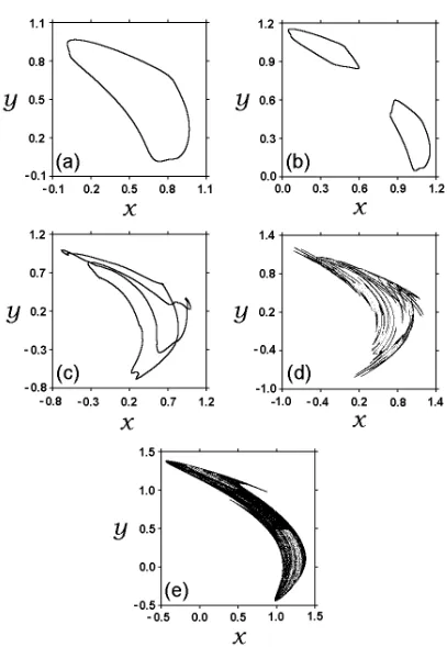
The examples of typical attractors of the map (1) are presented in Fig. 1. At a= 1.09, ε= 0.2 (here and hereafter we set b = 0.3) the attractor is a smooth closed invariant curve (“torus” T, Fig. 1(a)). With an increase of the nonlinearity parameter a, the torus T may bifurcate into a “double torus” 2T, which consists of a pair of smooth closed curves mapping into each other under iteration of the map, as shown in Fig. 1(b) wherea= 1.445,ε= 0.095. (Ifε is small enough, one can also observe a second torus-doubling bifurcation, which gives four smooth closed curves. Note, that the number of torus-doubling bifurcations on the route to chaos depends upon the quasiperiodic force amplitude ε; this number may increase and tend to infinity asε goes to zero [34]. The mechanism for the termination of torus-doubling cascades in invertible systems is discussed in Ref. [35].) On the other hand, a different kind of torus-doubling bifurcation (torus “length-doubling” bifurcation [29]) can occur for sufficiently large values of ε. This bifurcation produces a special type of torus, which is characterised by the existence of two wraps of a single invariant curve; we will refer it to as a “double-wrapped torus” T2 (see Fig. 1(c) where a= 0.728, ε= 0.36). Strange nonchaotic
and chaotic attractors of the map (1) are presented in Fig. 1(d) (a = 0.94,ε = 0.312) and Fig. 1(e) (a= 1.6, ε= 0.135), respectively.
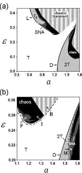
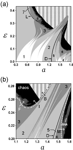
The phase diagram of the map (1) in the a− ε parameter plane (b = 0.3) is shown in Fig. 2(a). The regions of different types of dynamical behaviour are shown in different tones. Torus T (white), double torus 2T (light-grey), double-wrapped torus T2 (light-grey).
Regions of chaotic dynamics are shown in black. On the border between quasiperiodicity and chaos regions of SNA (dark-grey) exist. In the patterned area the map (1) has no attractor, and the trajectories go to infinity.
frac-talization of the smooth torus T [20]. The dotted line I corresponds to the intermittent mechanism of the birth of a SNA [23] via collision of torus T with a saddle chaotic invariant set [24]. The combined lineMcorresponds to the birth of a SNA via band-merging collision of a double torus 2T with a saddle parent torus [22]. A transition B from the region of quasiperiodicity to divergence of trajectories occurs when the torus T destroys and trans-forms into a chaotic transient via collision with a saddle chaotic set on the fractal basin boundary [26,27]. Arrows give the direction of movement in the parameter space for each transition to be observed.
III. PERTURBATION ANGLE DYNAMICS AND A SPECIAL CIRCLE
MAPPING
Let us take a smooth attracting torus of the map (1), given by invariant curve of the form
T{a,b} :{(x, y, θ)∈R2×T1|x=X{a,b}(θ), y =Y{a,b}(θ), θ∈ [0,2π)}. (2)
The pair of continuous and smooth functions{X{a,b}(θ), Y{a,b}(θ)}can be obtained by solving
the system of nonlinear functional equations
In what follows we can omit mention of the dependence of these functions upon the param-eters {a, b} and write simply {X(θ), Y(θ)}, although we should keep in mind the link of
{X(θ), Y(θ)}with the system (3).
Take a reference quasiperiodic trajectory {(xn, yn, θn)}n=0,1,...,∞ ∈ T, and consider a
perturbed trajectory close to it starting with the same initial phase: {(xn + δxn, yn +
δyn, θn)}n=0,1,...,∞. Evolution of a small perturbation δrn = (δxn, δyn)(n = 0,1, . . . ,∞)
Coordinatesxnandynin the map (4) are taken at the corresponding points of the trajectory
on the torus T: xn=X(θn), yn=Y(θn). For convenience, let us introduce terms
Now the map (4) can be rewritten as
δrn+1cosϕn+1 =−δrn[2X(θn) cosϕn+bsinϕn],
δrn+1sinϕn+1 =δrncosϕn,
θn+1 =θn+ 2πω (mod 2π),
(8)
and thus, eliminating the radius variable δr, we obtain
cotϕn+1 =−[2X(θn) +btanϕn],
θn+1 =θn+ 2πω (mod 2π).
(9)
In order to get an explicit map for the angle variable ϕ, one should take into account the conditions
ϕn∈[0, π/2)∪[3π/2,2π)⇒ϕn+1 ∈[0, π),
ϕn∈[π/2,3π/2)⇒ϕn+1 ∈[π,2π),
(10)
which immediately follow from the second equation of the system (8). Then, from (9) and (10) one can finally obtain the explicit mapping for the evolution of the perturbation angle variable ϕ:
Recall that X(θ) is a function of period 2π. The map (11) represents a kind of a circle mapping under external quasiperiodic forcing. Note, that attractors of the map (11) must be symmetric with respect to a shift π along the ϕ-axis. Therefore, the map (11) could be simplified to the form
ϕn+1 = arctan [2X(θn) +btanϕn] + (π/2),
θn+1 =θn+ 2πω (mod 2π),
Returning to the radial coordinate δr, one can see, that its dynamics is trivial. Indeed, for any small perturbation in a vicinity of the attracting torus T we immediately have:
δrn =
q
(δxn)2+ (δyn)2 ∼ exp (nλ1)
q
(δx0)2+ (δy0)2 =δr0exp (nλ1),
where λ1 < 0 is the largest nontrivial Lyapunov exponent, which characterizes stability of
the torus T.
The analysis of the dynamics of the perturbation angle ϕ on complex tori of the form kT (k = 2,4,8, . . .) in the map (1) requires trivial modification of the map (11). The last becomes cyclic:
ϕn+1 =f(ϕn, X(m)(θn)),
θn+1 =θn+ 2πω (mod 2π),
where n = kp+ m, p is integer, m = 1,2, . . . , k, and {X(m)(θ)} is a set of functions
determining a set ofk smooth closed curves which the complex toruskT consists of. On the other hand, for analysis of the dynamics of the perturbation angleϕ on the double-wrapped torus T2 it is convenient to redefine the phase variableθ on the interval [0,4π) and to rewrite
the map (11) in the following form:
ϕn+1 =f(ϕn, X(2)(θn)),
θn+1 =θn+ 2πω (mod 4π),
where X(2)(θ) is a function of the period 4π defining the double-wrapped torus T2.
IV. A LINK TO THE HARPER EQUATION
un+1 =−[un+ 2b−1/2X(θn)]−1,
θn+1 =θn+ 2πω (mod 2π).
(13)
Since the function X(θ) is 2π-periodic, it can be decomposed into Fourier series:
X(θ) =a0/2 +
the functional equation (3). For the case of small values of the quasiperiodic force amplitude ε (see the map (1)), one may take into account the first terms of the Fourier series only and obtain
which reduces to the Harper equation with a quasiperiodic potential after a standard change of the variables un =ψn−1/ψn:
ψn+1 +ψn−1+ 2λcos (2πωn+φ)ψn=Eψn, (17)
where φ=θ0+φ1 is a phase shift.
the following technique. Each dynamical regime of the map (16) was characterized by the non-trivial Lyapunov exponentσ and the phase sensitivity exponentδ[11]. These exponents take valuesσ = 0 andδ = 0 for a three-frequency torus,σ <0 andδ= 0 for a two-frequency torus, and σ <0 with δ >0 for the case of a SNA.
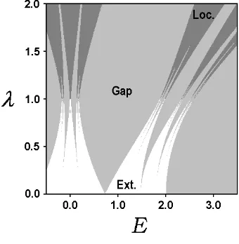
The link from the Harper equation to the map (11) suggests that the configuration of the phases on the diagram (Fig. 3) can be related to the structure of sets in the parameter space of the quasiperiodically forced H´enon map. Indeed, in the next section we will show that regions of different perturbation angle dynamics are organized as “tongues” of two- and three-frequency quasiperiodicity or of a complex behaviour corresponding to a SNA.
V. ANGULAR DYNAMICS OF PERTURBATIONS IN THE CONTEXT OF
TORUS BIFURCATIONS
Now we will focus on the angle dynamics of small perturbations in a vicinity of the torus T. Suppose we have a trajectory starting from the initial phaseθ0 on the torus and examine
its small perturbation with an arbitrarily chosen initial angle ϕ0. Further evolution of the
perturbation angle ϕ is determined by the map (11). In what follows, we choose a few sets of the parameters (a, ε) such that a smooth torus T exists in the map (1) and consider a dynamics of the map (11) at the same parameter values.
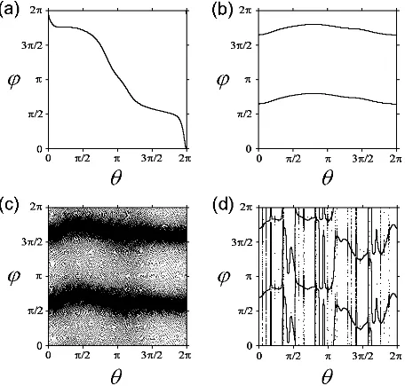
At a = 0.8, ε = 0.1 the attractor of the map (11) represents a smooth torus ϕ = Φ(θ) shown in Fig. 4(a). Note that tori of the map (11) may have different topology, demonstrate one or many wraps on the circle ϕ ∈ [0,2π) and consist of one or two segments, as shown in the Fig. 4(b) wherea= 1.3,ε= 0.5. The 2D map (11) is characterized by two Lyapunov exponents. A trivial Lyapunov exponent associated with the quasiperiodic variableθis equal to zero, while a nontrivial Lyapunov exponent in our cases takes the value σ=−0.1170 for the first set of parameter values andσ=−0.9755 for the second set. The angle variableϕnof
an arbitrarily chosen perturbation on the torus T asymptotically behaves as (ϕn−Φ(θn))∼
ϕn in our cases represents a regular two-frequency quasiperiodic motion.
As the parameters of the maps are varied toa= 0.85,ε= 0.077, the two-frequency torus of the map (11) disappears via the backward saddle-node bifurcation, and a three-frequency torus appears. A trajectory generated by the map (11) then uniformly fills a 2D torus
{ϕ ∈ [0,2π), θ ∈ [0,2π)} (see Fig.4(c)). Strictly speaking, in this situation the map (11) does not possess an attractor, since it is characterized by two zero Lyapunov exponents. Thus, the dynamics of the perturbation angleϕnis regular and represents a three-frequency
quasiperiodic motion.
On the other hand, as the parameters change to a = 0.9, ε = 0.28, the two-frequency torus of the map (11) destroys via phase-dependent mechanism with the birth of a strange nonchaotic attractor shown in Fig. 4(d). Note that the nontrivial Lyapunov exponent re-mains negative (σ =−0.7747). The angle variableϕn of an arbitrarily chosen perturbation
in a vicinity of the torus T asymptotically behaves as (ϕn−Φ(θn)) ∼exp(σn) as n → ∞,
where Φ(θ) is a fractal-like function characterized by non-differentiability and upper/lower semicontinuity [4]. As a result, the dynamics of the perturbation angle ϕn is irregular. A
graphic image of such dynamics is a trajectory on a strange nonchaotic attractor of the map (11).
In order to observe a configuration of regions corresponding to different types of dynamics of the perturbation angle variable ϕ in the a−ε parameter plane we need to combine the results obtained for the attractors of the maps (1) and (11). Such a combined phase diagram is presented in Fig. 5(a). The regions of chaos, SNA and chaotic transient in the map (1) are shown in black, dark-grey and pattern, respectively (the same as in Fig. 2(a)). The regions of the existence of a smooth attractor (i.e. T, 2T and T2 ) of the map (1) are subdivided
of the diagram in the region of complex dynamical transitions in the model map (1) is shown in Fig. 5(b).
From Fig. 5(a) one can see that the configuration of regions of different behaviour ofϕ is rather specific. The regions of a two- or three-frequency quasiperiodicity and of a SNA are organized as Arnold tongues. Recall that analogous tongues of the localized and extended phases were observed for the Harper equation (Fig. 3). However, the shapes of the tongues in Fig. 5(a) are distorted compared with those in Fig. 3. This distortion is associated with the non-rigorous transition from the Eq. (13) to Eq. (15), where only first terms of the Fourier series (14) were taken into account.
The line D (T → 2T) on the phase diagrams (Fig. 5(a),(b)) correspond to the usual torus-doubling bifurcation in the map (1). The line L (T→ T2) denotes the torus
length-doubling bifurcation, which leads to the birth of a double-wrapped torus T2. The lines
F, I, M and B in Fig. 5(b) denote the same dynamical transitions on the exit from the quasiperiodicity region that in Fig. 2(b).
On the other hand, the lines of regular bifurcations such as torus doubling (D) and torus length-doubling (L) separate regions shown in light-gray tone corresponding to the existence of two-frequency quasiperiodic dynamics of the perturbation angle variable ϕ. Note, that regular tori bifurcations have phase-independent character (for instance see Ref. [13]). Thus, numerical analysis shows that phase-independent bifurcations of tori in the model map (1) are accompanied by regular behavior of small perturbations on a torus.
In our opinion, the connection between the behaviour of perturbations on a torus and the types of torus bifurcations is a problem of significant mathematical interest. Recently, two of us (Jalnine and Osbaldestin) suggested a partial solution of this problem for the case of torus-doubling bifurcation [35]. We introduced Lyapunov vectors as basis directions of contraction for an element of phase volume in a vicinity of the torus and shown that torus-doubling can occur only if the dependence of the Lyapunov vectors upon the angle coordinate θ on torus is smooth. We have also shown that the appearance of a non-smooth dependence of the Lyapunov vectors upon the angle coordinate on torus terminates the line of torus-doubling bifurcation on the parameter plane. Note that, after sufficiently large number of iterations, an arbitrarily chosen initial perturbation vector of the form δr0 = (δx0, δy0,0)
VI. CONCLUSION
In the present work we investigated the dynamics of small perturbations of trajecto-ries on an attracting torus in the quasiperiodically forced H´enon map. We have shown that dynamics of the angle variable of a perturbation may be a two- or three-frequency quasiperiodicity, or it may have irregular character. In the last case the graphic image of such dynamics is a trajectory on a strange nonchaotic attractor. It was also shown that the appearance of irregular character in the approach of trajectories to an attracting torus precedes the destruction of such a torus via phase-dependent mechanisms with the birth of a strange nonchaotic attractor or of a chaotic transient.
ACKNOWLEDGMENTS
REFERENCES
[1] C. Grebogi, E. Ott, S. Pelikan, J. A. Yorke, Physica D 13, 261 (1984).
[2] M. Ding, C. Grebogi, E. Ott, Phys. Lett. A 137, 167 (1989).
[3] B. R. Hunt, E. Ott, Phys. Rev. Lett. 87, 254101 (2001).
[4] J. Stark, Physica D109, 163 (1997).
[5] G. Keller, Fundamenta Mathematicae 151, 139 (1996).
[6] S.P. Kuznetsov, A.S. Pikovsky, U. Feudel, Phys. Rev. E 51, R1629 (1995).
[7] A. Pikovsky, U. Feudel, J. Phys. A: Math. Gen. 27, 5209 (1994).
[8] A. S. Pikovsky, M. A. Zaks, U. Feudel, J. Kurths, Phys. Rev. E52, 285 (1995).
[9] U. Feudel, A. Pikovsky, A. Politi, J. Phys. A: Math. Gen. 29, 5297 (1996).
[10] J. W. Shuai, K. W. Wong, Phys. Rev. E57, 5332 (1998).
[11] A. Pikovsky, U. Feudel, CHAOS5, 253 (1995).
[12] K. Kaneko, Prog. Theor. Phys. 69, 1806 (1983).
[13] H. Broer, G. B. Huitema, F. Takens, B. L. J. Braaksma, Mem. Amer. Math. Soc.83, 1 (1990).
[14] P. R. Chastell, P. A. Glendinning, J. Stark, Phys. Lett. A 200, 17 (1995).
[15] P. Glendinning, Discrete and Continuous Dynamical Systems - Series B Vol. 6, No 4, P. 1 (2002).
[16] H. Daido, Prog. Theor. Phys. 71, 402 (1984).
[17] U. Feudel, A. S. Pikovsky, J. Kurths, Physica D88, 176 (1995).
[18] H. Osinga, J. Wiersig, P. Glendinning, U. Feudel, Int. J. of Bifurcations and Chaos Vol.
[19] S. P. Kuznetsov, Phys. Rev. E 65, 066209 (2002).
[20] T. Nishikawa, K. Kaneko, Phys. Rev. E 54, 6114 (1996).
[21] S. Datta, R. Ramaswamy, A. Prasad, Phys. Rev. E 70, 046203 (2004).
[22] J. F. Heagy, S. M. Hammel, Physica D 70, 140 (1994).
[23] A. Prasad, V. Mehra, R. Ramaswamy, Phys. Rev. Lett. 79, 4127 (1997).
[24] S.-Y. Kim, W. Lim, E. Ott, Phys. Rev. E 67, 056203 (2003).
[25] T. Yalcinkaya, Y.-C. Lai, Phys. Rev. Lett. 77, 5039 (1996).
[26] H. M. Osinga, U. Feudel, Physica D 141, 54 (2000).
[27] S.-Y. Kim, W. Lim, Phys. Lett. A 334, 160 (2005).
[28] O. Sosnovtseva, U. Feudel, J. Kurths, A. Pikovsky, Phys. Lett. A 218, 255 (1996).
[29] J. Heagy, W. L. Ditto, J. Nonlinear Sci.1, 423 (1991).
[30] J. J. Stagliano, J.-M. Wersmger, E. E. Slaminka, Physica D 92, 164 (1996).
[31] A. Witt, U. Feudel, A. S. Pikovsky, Physica D109, 180 (1997).
[32] A. Prasad, R. Ramaswamy, I. I. Satija, N. Shah, Phys. Rev. Lett. 83, 4530 (1999).
[33] S. S. Negi, A. Prasad, R. Ramaswamy, Physica D 145, 1 (2000).
[34] S. P. Kuznetsov, JETP Lett.39, 113 (1984).
FIGURES
FIG. 1. The typical attractors of the map (1): (a) torus T, (b) double torus 2T, (c)
FIG. 2. (a) The phase diagram of the map (1). (b) An enlarged fragment of the same diagram
FIG. 4. Attractors of the map (11) as graphic images of the dynamics of the perturbation
FIG. 5. The combined phase diagram of the maps (1) and (11). See text of the Sec. V for details.