076 Estimation Of Current Population Variance In Successive Sampling
Muhammad Azam, Qamruz Zamanand K. P. Pfeiffer
627 – 644
079 On The Long Memory Properties Of Emerging Capital Market: Evidence From Kuala Lumpur Stock Exchange
Turkhan Ali Abdul Manap and Salina Hj. Kassim
645 – 657
081 A State Space Model In Small Area Estimation
Kusman Sadik and Khairil Anwar Notodiputro
658 – 662
083 Comparison Cox Regression And Parametric Models In Survival Of Patients With Gastric Carcinoma
Mohamad Amin Pourhoseingholi, Ebrahim Hajizadeh, Azadeh Safaee, Bijan Moghimi Dehkordi, Ahmad Reza Baghestani and Mohammad Reza Zali
663 – 671
084 Run Test For A Sequence Of More Than Two Type Of Elements; An S-Plus Macro
Baghestani AR, Faghihzade S, Pourhoseingholi MA, Asghari M and Yazdani J
672 – 678
085 Association Between Duration Of Reflux And Patient Characteristics: A Quantile Regression Analysis
Mohamad Amin Pourhoseingholi, Soghrat Faghihzadeh, Afsaneh Zarghi, Manijeh Habibi, Azadeh Safaee, Fatemeh Qafarnejad and Mohammad Reza Zali
679 – 689
086 Evaluating Consensus Differentials Among Major Ethnics In Malaysia Via Fuzzy Logics
Puzziawati Ab Ghani and Abdul Aziz Jemain
690 – 700
088 Inefficiencies From Financial Liberalization: Some Statistical Evidence From Malaysia Using Social Cost Benefit Analysis
Yee Chow Fah and Tan Eu Chye
701 – 735
089 Risk Scoring System For Prediction Of Abdominal Obesity In An Iranian Population Of Youths: CASPIAN Study
Sayed Mohsen Hosseini , Roya Kelishadi and Marjan Mansourian.
736 – 744
090 Finding Critical Region For Testing The Presence Of Additive Outlier (AO) In GARCH(1,1) Processes By The Method Of Simulation
Siti Meriam binti Zahari and Mohamad Said Zainol
745 – 752
092 Comparison Of Model Selection Criteria In Determining The Best Mathematical Model
Zainodin Hj. Jubok, Ho Chong Mun, Noraini Abdullah and Goh Cheng Hoe
A State Space Model in Small Area
Estimation
Kusman Sadik1 and Khairil Anwar Notodiputro2
Department of Statistics Bogor Agricultural University / IPB Jl. Raya Dramaga, Bogor, Indonesia 16680
Abstract
There have been two main topics developed by statisticians in a survey, i.e. sampling techniques and estimation methods. The current issues in estimation methods relate to estimation of a particular domain having small size of samples or, in more extreme cases, there are no sample available for direct estimation (Rao, 2003). There is a growing demand for reliable small area statistics in order to asses or to put into policies and programs. Sample survey data provide effective reliable estimators of totals and means for large area and domains. But it is recognized that the usual direct survey estimator performing statistics for a small area, have unacceptably large standard errors, due to the circumtance of small sample size in the area. In fact, sample sizes in small areas are reduced, due to the circumtance that the overall sample size in a survey is usually determined to provide specific accuracy at a macro area level of aggregation, that is national territories, regions and so on. The most commonly used models for this case, usually in small area estimation, are based on generalized linear mixed models (GLMM). It is happened some time that some surveys are carried out periodically so that the estimation could be improved by incorporating both the area and time random effects. In this paper we propose a state space model which accounts for the two random effects and is based on two equation, namely transition equation and measurement equation.
Key words: direct estimation, indirect estimation, small area estimation (SAE), general linear mixed model (GLMM), empirical best linear unbiased prediction (EBLUP), block diagonal covariance, Kalman filter, state space model.
1. Introduction
The problem of small area estimation is how to produce reliable estimates of area (domain) characteristics when the sample sizes within the areas are too small to warrant the use of traditional direct survey estimates. The term of small area usually denote a small geographical area, such as a county, a province, an administrative area or a census division. From a statistical point of view the small area is a small domain, that is a small sub-population constituted by specific demographic and socioeconomic group of people, within a
1
2
658
larger geographical areas. Sample survey data provide effective reliable estimators of totals and means for large areas and domains. But it is recognized that the usual direct survey estimators performing statistics for a small area, have unacceptably large standard errors, due to the circumstance of small sample size in the area. In fact, sample sizes in small areas are reduced, due to the circumstance that the overall sample size in a survey is usually determined to provide specific accuracy at a macro area level of aggregation, that is national territories, regions ad so on (Datta and Lahiri, 2000).
Demand for reliable small area statistics has steadily increased in recent years which prompted considerable research on efficient small area estimation. Direct small area estimators from survey data fail to borrow strength from related small areas since they are based solely on the sample data associated with the corresponding areas. As a result, they are likely to yield unacceptably large standard errors unless the sample size for the small area is reasonably large(Rao, 2003). Small area efficient statistics provide, in addition of this, excellent statistics for local estimation of population, farms, and other characteristics of interest in post-censual years.
2. Indirect Estimation in Small Area
A domain (area) is regarded as large (or major) if domain-specific sample is large enough to yield direct estimates of adequate precision. A domain is regarded as small if the domain-specific sample is not large enough to support direct estimates of adequate precision. Some other terms used to denote a domain with small sample size include local area, sub-domain, small subgroup, sub-province, and minor domain. In some applications, many domains of interest (such as counties) may have zero sample size.
In making estimates for small area with adequate level of precision, it is often necessary to use indirect estimators that borrow strength by using thus values of the variable of interest,
y, from related areas and/or time periods and thus increase the effective sample size. These values are brought into the estimation process through a model (either implicit or explicit) that provides a link to related areas and/or time periods through the use of supplementary
information related to y, such as recent census counts and current administrative records
(Pfeffermann 2002; Rao 2003).
Methods of indirect estimation are based on explicit small area models that make specific allowance for between area variation. In particular, we introduce mixed models involving random area specific effects that account for between area variation beyond that explained by auxiliary variables included in the model. We assume that Ti = g(Yi) for some
specifiedg(.) is related to area specific auxiliary data zi = (z1i, …, zpi)T through a linear model
Ti = ziTE + bivi, i = 1, …, m
where the bi are known positive constants and E is the px1 vector of regression coefficients.
Further, the vi are area specific random effects assumed to be independent and identically
distributed (iid) with
Em(vi) = 0 and Vm(vi) = Vv2 (t 0), or via iid (0, Vv2)
3. Generalized Linear Mixed Model
Datta and Lahiri (2000), and Rao(2003) considered a general linear mixed model (GLMM) covering the univariate unit level model as special cases:
yP = XPE+ZPv + eP
Random vectors v and eP are independent with eP a N(0,V2\P) and v a N(0,V2D(O)), where \P is a known positive definite matrix and D(O) is a positive definite matrix which is
components of the form Vi2/V2. Further, XPandZP are known design matrices and yP is the N
where the asterisk (*) denotes non-sampled units. The vector of small area totals (Yi) is of the
form Ay + Cy* with A = im nT and C = where = blockdiag(A G, the BLUP (best linear unbiased prediction) estimator of P is given by (Rao, 2003)
H
P~ = t(G,y) = 1TE~ + mT~v = 1TE~ + mTGZTV-1(y - XE~)
Model of indirect estimation, Tˆi ziTE + bivi + ei, i = 1, …, m, is a special case of
GLMM with block diagonal covariance structure. Making the above substitutions in the general form for the BLUP estimator of Pi, we get the BLUP estimator of Ti as:
4. State Space Models
Many sample surveys are repeated in time with partial replacement of the sample elements. For such repeated surveys considerable gain in efficiency can be achieved by borrowing strength across both small areas and time. Their model consist of a sampling error model
Tˆit Tit + eit, t = 1, …, T;i = 1, …, m Tit = zitTEit
where the coefficients Eit = (Eit0,Eit1, …, Eitp)T are allowed to vary cross-sectionally and over
time, and the sampling errors eit for each area i are assumed to be serially uncorrelated with
mean 0 and variance \it. The variation of Eit over time is specified by the following model:
p
It is a special case of the general state-space model which may be expressed in the form
yt = ZtDt + Ht; E(Ht) = 0, E(HtHtT) = 6t
Dt = HtDt-1 + AKt; E(Kt) = 0, E(KtKtT) = *
where Ht and Kt are uncorrelated contemporaneously and over time. The first equation is
known as the measurement equation, and the the second equation is known as the transition equation. This model is a special case of the general linear mixed model but the state-space form permits updating of the estimates over time, using the Kalman filter equations, and smoothing past estimates as new data becomes available, using an appropriate smoothing algoritm.
is the covariance matrix of the prediction errors at time (t-1). At time t, the predictor of Dt and
its covariance matrix are updated using the new data (yt,Zt). We have yt - ZtĮt|t-1
~ = Z
t(Dt- Įt|t-1) + H
~
t
which has the linear mixed model form with y = yt - ZtĮt|t-1
~ ,Z = Z
t,v = Dt- Įt|t-1
~ ,G = P
t|t-1
and V = Ft, where Ft = ZtPt|t-1ZtT + 6t. Therefore, the BLUP estimator v~= GZTV-1y reduces
to
-1 t
Į
~ =
-1 t | t
Į
~ + P
t|t-1ZtTFt-1(yt - ZtĮt|t-1
~ )
5. Case Study
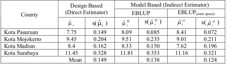
Model of small area estimation can be applied to estimate the average of households expenditure per month for each of m = 37 counties in East Java, Indonesia. We used Susenas data (National Economic and Social Survey, BPS 2003-2005) to demonstrate the performance of EBLUP resulted from state space models .
Table 1. Design Based and Model Based Estimates of County Means and Estimated Standard Error
Model Based (Indirect Estimator) Design Based
(Direct Estimator) EBLUP EBLUP(state space)
County
i
Pˆ s(Pˆi ) H
i
Pˆ s(PˆHi )
ss i
Pˆ s( ss )
i
Pˆ
Pacitan 4.89 0.086 3.89 0.062 5.23 0.038
Ponorogo 5.5 0.148 5.83 0.149 5.73 0.132
Trenggalek 5.3 0.135 6.89 0.155 5.65 0.161
Tulungagung 6.78 0.229 7.06 0.215 7.05 0.172
Blitar 5.71 0.132 5.74 0.198 6.12 0.141
Kediri 5.62 0.105 7.09 0.110 6.45 0.091
Malang 5.94 0.128 6.58 0.112 5.19 0.109
Lumajang 5.07 0.119 4.75 0.118 5.74 0.081
Jember 4.65 0.090 4.96 0.126 5.28 0.113
Banyuwangi 5.98 0.142 5.55 0.124 6.15 0.131
Bondowoso 4.53 0.127 4.64 0.092 5.43 0.105
Situbondo 4.67 0.104 5.89 0.085 4.44 0.074
Probolinggo 5.54 0.154 6.07 0.184 7.34 0.186
Pasuruan 6.31 0.151 4.95 0.121 6.39 0.109
Sidoarjo 9.33 0.169 9.46 0.177 8.32 0.123
Mojokerto 6.91 0.160 6.55 0.135 8.25 0.107
Jombang 6.09 0.131 5.06 0.130 5.96 0.091
Nganjuk 5.56 0.125 4.40 0.041 4.87 0.029
Madiun 5.5 0.139 5.16 0.116 5.46 0.121
Magetan 5.52 0.161 4.84 0.145 4.16 0.132
Ngawi 4.89 0.102 4.61 0.097 4.15 0.086
Bojonegoro 5.06 0.093 5.25 0.067 4.50 0.047
Tuban 6.02 0.114 5.75 0.061 6.47 0.046
Lamongan 6.29 0.106 6.47 0.123 5.69 0.065
Gresik 8.49 0.186 9.07 0.167 9.01 0.198
Bangkalan 6.61 0.140 5.69 0.091 7.00 0.076
Sampang 6.32 0.158 7.20 0.150 6.85 0.182
Pamekasan 5.78 0.107 6.10 0.126 5.93 0.109
Sumenep 5.48 0.108 5.76 0.077 5.09 0.032
Kota Kediri 8.01 0.159 7.60 0.157 7.11 0.144
Kota Blitar 7.98 0.191 7.63 0.159 8.51 0.182
Kota Malang 11.14 0.298 12.63 0.273 11.61 0.225
Model Based (Indirect Estimator) Design Based
(Direct Estimator) EBLUP EBLUP(state space)
County
i
Pˆ s(Pˆi ) H
i
Pˆ s( ) Pˆiss
H i
Pˆ s( ss )
i
Pˆ
Kota Pasuruan 7.75 0.149 8.09 0.085 8.41 0.072
Kota Mojokerto 9.45 0.204 9.51 0.235 9.01 0.211
Kota Madiun 8.4 0.162 8.33 0.150 7.62 0.196
Kota Surabaya 11.45 0.328 11 1 .8 0.353 .111 6 0.321
Mean 0.149 0.138 0.124
Table 1 shows the design based and model based estimates. The design based estimates
is direct estimator based on sampling design. EBLUP estimates, H
i
Pˆ , used small area model with area effects (data of Susenas 2005) whereas, EBLUP(ss) estimates, Pˆiss, used small area
model with area and tim effec (data of enas 2003 to 2005). The estimated standard
errors are denoted by s(Pˆ ), s(i H i
Pˆ ), and s( ss i
Pˆ ). It is clear from Table 1 that the estimated standard errors of mean for the model based is less than the estimated standard error for the
e ts Sus
estimates design based. The estimated standard error mean of EBLUP(ss) is less than EBLUP.
6.
etermination of suitable linking models are crucial to the formation of indirect estimators.
7.
q
tors (BLUP) in Small Area Estimation Problems,
q New Developments and
q
versity of
Conclusion
Small area estimation can be used to increase the effective sample size and thus decrease the standard error. For such repeated surveys considerable gain in efficiency can be achieved by borrowing strength across both small area and time. Availability of good auxiliary data and d
Reference
Datta, G.S, and Lahiri, P. (2000). A Unified Measure of Uncertainty of Estimated Best Linear Unbiased Predic
Statistica Sinica,10, 613-627.
Pfeffermann, D. (2002). Small Area Estimation – Directions.International Statistical Review,70, 125-143.
Pfeffermann, D. and Tiller, R. (2006). State Space Modelling with Correlated Measurements with Aplication to Small Area Estimation Under Benchmark Constraints. S3RI Methodology Working Paper M03/11, Uni
Southampton. Available from: http://www.s3ri.soton.ac.uk/publications.
q Rao, J.N.K. (2003). Small Area Estimation. John Wiley & Sons, Inc. New Jersey. Rao, J.N.K., dan Yu, M. (1994). Small Area Estimation by Combining Time Series
and Cross-Sectional Data. Procee
q
dings of the Section on Survey Research Method.
q
ating the Variance of Generalized Regression Estimator. Biometrika,76,
527-q Thompson, M.E. (1997). Theory of Sample Surveys. London: Chapman and Hall.
American Statistical Association.
Swenson, B., dan Wretman., J.H. (1992). The Weighted Regression Technique for Estim
537.
662