A SAS/IML program for simulating pharmacokinetic
data
Estelle Russek-Cohen
a,1,Marilyn N. Martinez
b,∗,Anna B. Nevius
baDepartment of Animal and Avian Sciences, University of Maryland, College Park, MD 20742, USA bCenter for Veterinary Medicine, US Food and Drug Administration, 7500 Standish Place, Rockville,
MD 20855, USA
Received 21 July 2004; received in revised form 6 October 2004; accepted 19 October 2004
KEYWORDS
Monte Carlo simulation; SAS;
Bioequivalence; Population kinetics; Veterinary
pharmacokinetics
Summary Data simulation can be an invaluable tool for optimizing the design of bioequivalence trials. It can be particularly useful when exploring alternative ap-proaches for assessing product comparability especially in the context of encounter-ing various complex experimental situations that can occur in veterinary medicine. With this in mind, we designed a novel SAS/IML program to generate pharmacoki-netic datasets that reflect the various kipharmacoki-netic, population, and study design charac-teristics that complicate the bioequivalence evaluation of animal health products. Developing this simulation program within SAS provides an opportunity to utilize the statistical capabilities of this software platform.
Published by Elsevier Ireland Ltd.
1. Introduction
Traditionally, product bioequivalence determina-tions are rooted in the use of blood level metrics that reflect the rate and extent of drug absorp-tion. As stated in the Food and Drug Administration Center for Veterinary Medicine (FDA CVM) Guidance #35 [1], these attributes are most frequently de-scribed by the observed peak drug concentration (Cmax) and the area under the concentration ver-sus time curve (AUC). More recently, exposure
con-*Corresponding author. Tel.: +1 301 827 7577.
E-mail addresses: [email protected] (E. Russek-Cohen), [email protected] (M.N. Martinez), [email protected] (A.B. Nevius).
1 Tel.: +1 301 405 1403; fax: +1 301 405 7980.
cepts have gained acceptance as the perspective from which to consider product comparability[2]. In this regard, the same bioavailability parameters (AUC andCmax) are used but are considered mea-sures of the extent of systemic exposure and peak exposure, respectively.
Whether dealing with human or veterinary phar-maceuticals, several challenging issues can com-plicate the evaluation of product bioequivalence. While product bioequivalence trials in human and veterinary medicine share many of the same sta-tistical and study design attributes, there are also many unique challenges confronted within the framework of veterinary medicine. For exam-ple, difficulties arise when assessing the relative bioavailability of products delivered in feed and water. In these situations, drug intake is
tially random, being dependent upon the feed-ing behavior of the animal. Gavage dosfeed-ing, while useful to demonstrate the impact of the dosage form on product bioavailability, does not provide information on product palatability and other con-sumption variables. Investigators can control the time when the drug is introduced or removed, but cannot control when the drug is consumed. In these situations, the development of an opti-mal blood sampling strategy[3]can be enormously challenging.
The presence of multiple absorption maxima can also complicate bioavailability comparisons. These complex profiles may be attributable to factors such as enterohepatic recirculation[4], gastric drug retention and gastric motility cycles[5,6] and ion trapping[7]. Apparently random peaks and troughs are also associated with certain long-acting im-plants, such as those containing the growth pro-motants zeranol[8]and trenbolone[9]. These prod-ucts can release drug for periods exceeding 90 days, during which time huge fluctuations in serum drug concentrations can occur. Assessing the bioequiva-lence of these products is problematic because no singular absorption rate constant or peak exposure can be defined.
Large variability in treatment effects is often observed when a parallel rather than a crossover study design is employed. In these cases, the population distribution characteristics of pharma-cokinetic parameter values can strongly influence the bioequivalence assessment. Within veterinary medicine, parallel study designs are needed when treatments are administered to growing animals (where substantial physiological changes can oc-cur, thereby biasing period 1 versus 2 treatment comparisons), when the products are associated with very long residence times (e.g., implants), and when an animal’s blood volume is limited (e.g., fish and poultry). Furthermore, confounding the evalu-ation parallel design bioequivalence studies are oc-casions when subpopulations exhibit markedly dif-ferent drug pharmacokinetic characteristics. These subpopulations may be defined by differences in drug clearance or volume of distribution, both be-ing formulation-independent effects. For example, within veterinary species, differences in drug phar-macokinetics have been observed between breeds of dogs [10,11], chickens [12,13] sheep [14], and cattle[15]. Pharmacokinetics can also be affected by animal age, sex, and diet [15—17]. Such vari-ations are not a concern if a crossover study de-sign is employed and if there are no subject-by-formulation interactions.
With regard to subject-by-formulation interac-tions, while this possibility and its therapeutic
sig-nificance has been widely discussed [18], there are few examples where they have actually been observed. One known example is the subject-by-treatment interaction seen when the bioavailabil-ity of certain earlier formulations of diazepam were compared to Valium[19]. In this case, human sub-jects with low gastric acidity had difficulty absorb-ing generic diazepam formulations, but such prob-lems were not observed in subjects with normal gastric acidity. Therefore, the generic and inno-vator diazepam formulations were bioequivalent in normal healthy volunteers but inequivalent in achlorhydric subjects.
To explore the influence of the aforementioned kinds of concerns on bioequivalence determina-tions, Monte Carlo simulation methods are fre-quently employed (e.g., [20—24]). The use of in silico techniques provides an inexpensive venue for evaluating the relationship between study at-tributes, the pharmacokinetics of a compound, and the sensitivity of a bioequivalence determination to changes in either study design or kinetic assump-tions. As with any in silico examination, conclu-sions are a function of the basic model assumptions (such as the pharmacokinetic model), the shape of the distribution of the pharmacokinetic param-eters, the magnitude of the variability about each of these parameters, and the covariance structure of the model parameters.
Fig. 1 Basic pharmacokinetic models and corresponding parameters used in developing the SAS pharmacokinetics simulation program.
In contrast with other simulation programs, we provide open source code so that users may modify the program to meet their particular need. Thus, a user may wish to compare existing and novel ap-proaches to the evaluation of bioequivalence while another user may be more focused on traditional comparisons of drug formulations.
Based upon our evaluation of bioequivalence study datasets that have been submitted to FDA/CVM, we have identified a number of condi-tions that can complicate the design and analysis of these trials. Using SAS programming language, we have developed a tool for exploring the conse-quences of these various challenges. This project reflects a first stage in our efforts to explore the performance of alternative metrics for evaluating product bioequivalence.
2. Computational methods and theory
The simulation software program allows for the use of either a one- or two-compartment open body model [25]. In both cases, drug enters and leaves from the central (blood) compartment. More complex pharmacokinetic scenarios, such as three-compartment mamillary models [26] are not be-ing considered since one- and two-compartmental models describe the clinically relevant portion of the concentration/time profile of most compounds. Both the one- and two-compartment open body models contain a single input rate constant (Ka) and a single output rate constant (Kel). Instan-taneous (intravenous) administration can be sim-ulated by setting the mean Ka value to an ex-tremely large number (e.g., 1000), with zero vari-ability. The fundamental difference between a one and two compartment open body model is that the two-compartment model includes rate constants describing the partitioning of the drug between
blood (central compartment) and some hypothet-ical ‘‘peripheral’’ (or tissue) compartment. The in-tercompartmental rate constants (kcp andkpc) de-scribe the movement of drug between blood and tissue (Fig. 1).
While rate constants have been described as both lettered and numbered variables through-out the pharmacokinetic literature (whereKa=K01,
Kel=K10, kcp=k12 and kpc=k21), only lettered nomenclature is used in this SAS program.
The user specifies the terms that drive the model. This includes values for parameter means, variances, and parameter correlation matrices for the test and reference groups. Each of these model-ing components are defined separately for the test and reference products, allowing for a comparison not only of formulation effects but also of physi-ological variables that can affect such basic phar-macokinetic parameters as volume and clearance. Thus, the definitions of treatments 1 and 2 need not be restricted to the comparison of two formu-lations but can be expanded to compare drug ex-posure characteristics across conditions that may alter patient physiology. This latter point can be particularly important when comparing blood level profiles across target animal species, a comparison often used to provide substantial evidence of effec-tiveness for product use in a minor animal species, such as goats, sheep, and wildlife[27].
‘‘t’’ (Ct) is defined as follows[25,28]:
F is the percent of dose actually absorbed and
Vc is the dilution factor estimating the fluid vol-ume of the blood (central) compartment within which the administered dose distributes. For a one-compartment model, Vc represents the en-tire distribution volume of the body. For a two-compartment model,Vc represents the volume of distribution associated with the central compart-ment. The total distribution volume is the summa-tion of central and peripheral compartments, and is represented by the equilibrium volume parameter, volume of distribution at steady state[28].
˛= 1
When the user selects a one-compartment body model, ˛ and kpc are automatically set to equal zero. By settingkpcand˛to zero, then
which simplifies to 1
Ka−ˇ (8)
which simplifies to −1
Ka−ˇ (10)
Thus, with ˛ and kpc set to zero, the two-compartment model (Eq.(1)) can be written as:
Ct=
Since, in a one-compartment model, ˇ is the same asKeland Vcis the same asV, the equation for a one-compartment open body model can be written as:
Ct=
F×Ka×D
V(Ka−Kel) ×(exp
−Kel×t−exp−Ka×t) (12)
It should be noted thatkcpvalues are not specified by the user. This is because values ofkcpare auto-matically set by the values of˛,ˇ,kpc, andKeldue to the relationship[25]:
kcp=˛+ˇ−kpc−Kel (13)
In future iterations of this program, the absorption component will be modified to allow for the inclu-sion of an inverse Gaussian model to describe the input function as a bell shaped curve that asymp-totically approaches zero[29].
We establish that the population covariance ma-trix for each treatment group is positive definite by checking to see that its determinant is positive. The assumption of positive definite is essential for sub-sequent statistical calculations. If the determinant is less than or equal to zero, an error message is printed in the output and the simulation is termi-nated. Usually, the correlation matrix is the source of this problem and the user will need to think about alternative values for this matrix. Correlations that are too high may be a possible issue.
The determination of product bioequivalence is based upon the use of TOST or a two one-sided tests procedure [30]. This hypothesis can be stated as follows[30], where R is the reference product and T is the test product:
H0.
T−R≤ −0.20RorT−R≥0.20R (14) H1.
−0.20R< T<0.20R (15)
Similarly, when considering ln-transformed data, the interval hypothesis can be stated as follows:
H0.
T
R ≤0.80 or T
H1.
0.80< T R
<1.25 (17)
Assuming that a parallel study design is used to compare the untransformed values associated with the test (T) and reference (R) treatments, the con-fidence intervals about the difference in treatment means are estimated as follows:
L=(¯XT−X¯R)− in the upper tail of the Student’st-distribution with
v degrees of freedom, where v= (nT−1) + (nR−1) for a parallel design study, and˛= 0.05 per tail.
To express these intervals relative to the ref-erence means, the lower limit (Lu) and the up-per limit (Uu) about the difference in the untrans-formed means of treatment pharmacokinetic pa-rameter values (e.g., AUC andCmax) are estimated as follows:
Two formulations are considered bioequivalent when Lu≥ −0.20 and Uu≤0.20. When the phar-macokinetic parameter values are ln-transformed (and we assume that in Eqs.(18)and(19)we have used the means and standard deviations of the ln-transformed data), then the lower (Lt) and upper (Ut) confidence interval about the ratio of the treat-ment means is estimated as follows:
Lt=expL−1 (22)
Ut=expU−1 (23)
We consider parameters to be bioequivalent when
Lt≥ −0.20 andUt≤0.25.
When only one variable is compared (treatment), thet-test can be used to estimate the standard er-ror of the estimate of the difference between treat-ment means. Alternatively, the estimator,s2, which will be used in the calculation of the 90% confidence interval, can be obtained from the ‘‘error’’ mean square term found associated with an analysis of variance (ANOVA).
3. Program description
A simulation package was written in SAS/IML. The SAS software was selected for this project for four reasons:
1. It is used within CVM for the analysis of the bioe-quivalence datasets.
2. The program can be easily modified to meet the needs of the investigator.
3. The software is widely available and can be run on a desktop computer.
4. SAS output can be exported into a format com-patible with other software programs such as EX-CEL and WinNonLin (Pharsight). In this regard, the SAS datasets are saved within a user-defined directory (libname), allowing it to be copied onto a diskette or imported into other software programs. The user can also save the generated SAS datasets for comparison with future algo-rithms as they are developed.
SAS is capable of generating very large simulated datasets. By using pseudorandom number genera-tors, values can be generated that mimic the de-sired properties for a given dataset, and thousands of these datasets can be created. Each dataset can be viewed as the results of a single bioequivalence trial.
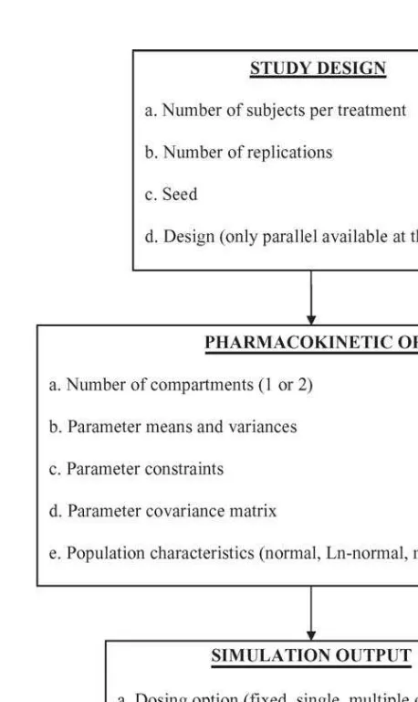
Considering the kinds of complex bioequivalence issues that arise within CVM, the simulation pro-gram provides users the flexibility to define a va-riety of modeling attributes, including pharmacoki-netic model and parameter values, the existence of subpopulations, fixed or random input, the popula-tion distribupopula-tion of each variable (ln-normal, nor-mal, or bimodal), the presence or absence of as-say noise, and the method of handling values that drop below the limit of quantification (LOQ) of the analytical method (Fig. 2). A summary of the various terms used in this program is provided in Appendix A.
3.1. Seeds
Fig. 2 Simulation decision tree: options provided in this SAS program.
of caution, an important limitation is that random number generators can potentially repeat a number sequence if the quantity of values to be generated exceeds 231. By using different seeds to generate data for each treatment or any subset of the data, the time until repeats occur can be substantially increased.
3.2. Study design
At this point in time, the programmer can only spec-ify a parallel study design. However, a future iter-ation of this program will allow for the simuliter-ation of crossover trials.
3.3. Pharmacokinetic model
Either a one- or two-compartment open body model can be selected:
1. ncompart=1: this indicates that a one-compartment model is selected. The user must define the mean and coefficient of variation for four parameters:Ka,Vc,F, andKel. In this case, the equation for a two-compartment model is used, but the values forkpc, kcp, and˛are set to zero.
2. ncompart=2: this indicates the use of a two-compartment model. The user must define means and coefficients of variation forKa,kpc,
Vc,˛,F, andˇ. The value ofkcpis automatically defined based upon Eq.(13).
Output parameters (e.g., AUC andCmax) can be evaluated as if they followed a normal or a log-normal distribution, and statistical tests can be run on the transformed or untransformed values. As currently written, the ln-transformed param-eter values are used for estimating the confi-dence intervals about the ratio of treatment means. Should the use of untransformed param-eter values be preferred, coding will need to be revised to accommodate corresponding changes in the equation for calculating confidence in-tervals about the difference in treatments ex-pressed relative to the reference mean[1].
3.4. Constraints on F
In most situations, it is biologically inappropriate for values of F(bioavailability) to exceed 100% of the administered dose. Therefore, the user has the option of using the following command to constrain the simulated output ofFfor the test preparation:
Note: F= paramt[i, 3]
if paramt[i,3]> =1then paramt[i,3] =1; if paramt[i,3]< = .001then paramt[i,3] = .001;
This command needs to be specified separately for the test and reference groups. The same state-ment can be used for the reference formulation by substituting paramr in place of paramt. This op-tion is included as a command within the SAS code. By inserting an asterisk immediately prior to these comments (*Note: F= paramt[i, 3]), the output will not constrainFto fall between 0.001 and 1.0.
If this parameter is simulated under the condi-tion of a lognormal distribucondi-tion, the code can be modified to read as follows:
Note:logF= paramt[i, 3]
if paramt[i,3]> =0then paramt[i,3] =0;
3.5. Population considerations
Randomly generated pharmacokinetic parameters can follow either a normal, a ln-normal, or a mix-ture of two normal distributions. While there are examples of simulated bioequivalence studies that are based upon normally distributed parameters [20,21,31], many investigators argue that pharma-cokinetic parameters (such as clearance and vol-ume of distribution) more closely follow a ln-normal distribution[32—34]. Differences in the simulation output resulting from the use of normal versus ln-normal parameter distributions is provided else-where[35]. Further arguments suggest that due to the presence of subpopulations, neither a normal nor a ln-normal distribution can accurately describe the pharmacokinetic parameters within a popula-tion. Jelliffe et al. [36] notes that many patient populations are composed of clusters of subpopu-lations, in which case neither the assumption of a normal nor ln-normal parameter distribution is ap-propriate.
The user is asked to define parameter distribu-tion characteristics as follow:
1. PARMTYPE= 0: single multivariate normal distri-bution within each treatment group. When simu-lations are conducted under the assumption that parameters are normally distributed, the user runs the risk of obtaining negative values for some parameters. To avoid generating negative parameter values, the output reminds the user that when large %CV values are specified, use of a ln-normal distribution (PARMTYPE= 1) may be more appropriate.
2. PARMTYPE= 1: single multivariate ln-normal population within each group. When conducting simulations under this condition, the parameter means and %CV must be expressed as the nat-ural log of the targeted values. To transform a CV from a normal distribution to one that ap-proximates the error associated with values gen-erated on a log scale, the following equation should be employed[37]:
cv(y)= v(y)
where cv(y) is the coefficient of variation ex-pressed on the linear scale,v(y) the variance of the untransformed data,m(y) the mean of the untransformed data,v(x) the variance of the ln-transformed data, andm(x) is the mean of the ln-transformed data.
To transform mean and variance estimates from the log scale to the linear scale, the following equations may be used:
cv(y′) where cv(y′) is the coefficient of variation ex-pressed on the linear scale based upon the back transformed data.
3. PARMTYPE= 2: the population is described as a mixture of two multivariate normal distributions or two subpopulations within each treatment. This option can be used to simulate populations that are bimodal.
For each of theNREPdatasets, a binomial ran-dom number generator is used to determine the number of individuals from each subpopulation that are included in the mixture. For example, pmix1=.9will result in a parameter distribution such that, on the average, 90% of the samples will follow the characteristics of the first or pri-mary subpopulation while 10% will be from the second subpopulation. This reflects the reality of random sampling of subjects in the presence of a mixture of two types of individuals. The only similarity between these subpopulations is that they share the same correlation matrix. Since a subpopulation can be defined for any parameter mean or variance, this subgroup can be as dif-ferent than or similar to the main population as desired. If a second subpopulation is to be simu-lated for one treatment but not for the other (for example, model conditions similar to that pre-viously described for diazepam), one treatment arm can have two subpopulations with identical means and variances whereas the second arm can have two distinct sets of means and vari-ances. In so doing, data within the treatment arm that has two identical subpopulations will follow a single multivariate normal distribution.
3.6. Measurement error
the opportunity to superimpose measurement error to each observation.
Within the regulatory arena, specific recommen-dations have been forwarded with regard to as-say performance[38]. For example, the guidance specifies that the error and the %CV should not ex-ceed 15%, except at the lower limit of quantifica-tion, where error and %CV should not exceed 20%. Based upon these recommendations, the program includes an option to define confidence limits about the ratio of the true versus observed values. The coding for this is as follows:
1. measerr=0: this implies that no measurement error will be added to the simulated drug con-centrations.
2. measerr=1: this implies that a multiplicative measurement error is added to each simulated drug concentration.
To have a 99% chance of obtaining ‘‘measured’’ values that fall between 80% and 125% of the true concentration, the coding would be as follows:
99% chance of being within 80% and 125% of the true concentration;
ptail = 1−(1−.99)/2;
zvalue = probit(ptail); logtop = log(1.25); *note ln(.8) =−logtop.
To specify greater error (e.g., 80% chance of falling within the limits of 70% and 143%, the coding would be modified as follows:
80% chance of being within 70% and 143% of the true concentration;
ptail = 1−(1−.80)/2;
zvalue = probit(ptail); logtop = log(1.43); *note ln(.7) =−logtop.
Alternatively, the user can modify this portion of the program to describe any type of error model deemed appropriate. For example, one can employ the more complex error models (e.g., quadratic equations) such as those described by Jelliffe et al. for the gentamycin emit assay [39]. The char-acteristics of the error pattern become particularly important when simulating the use of sparse blood samples, as may occur when studying fish or other small animal species. In these cases, where one or two samples represent the total information ob-tained on a particular subject, ignoring the pres-ence of a nonlinear error pattern (such as that asso-ciated with the emit assay) can result in the genera-tion of drug concentragenera-tions that incorrectly suggest the presence of multimodal distributions[40].
3.7. Setting the lower limit of
quantification
Validated analytical methods specify an LOQ be-low which the quantification of drug concentrations is deemed unreliable. Generally, CVM recommends that for single dose pharmacokinetic investigations, the AUC estimate should not extend beyond the last blood sampling time associated with drug concen-trations at or above the LOQ (AUC0—last). Therefore, this program is designed to allow the user to spec-ify an LOQ (coded as ‘‘loquant’’) that serves as the boundary at which AUC estimates are truncated (i.e., for generating AUC0—last). The use of this trun-cation can be valuable for determining the fre-quency and duration of blood samples, allowing the investigator to explore the percentage of the popu-lation that will have quantifiable concentrations out to the specified sampling time. Alternatively, the program allows for drug concentrations to be fac-tored into the AUC estimate as some specified value when the simulated concentrations drop below the LOQ. This option is coded as ‘‘lowlim’’. If selected, all concentrations falling below the ‘‘lowlim’’ are read as the concentration termed ‘‘lowlimv’’. For example, if the user wishes all concentrations that fall below the limit of 5g/mL to be factored into the AUC estimate as 1g/mL, the coding would be as follows:
lowlim = 5; lowlimv= 1;
The latter function should not be used when sim-ulating bolus administrations due to the error that can be introduced into the AUC estimates (i.e., profiles may be artificially extended well beyond the time when concentrations truly approach zero). However, this function may be valuable when sim-ulating conditions resulting in multiple peaks and troughs (e.g., when using the random input func-tion). By allowing for multiple simulations using the same seeds and parameter estimates, the investiga-tor can determine ways to optimize blood sampling times and to minimize the bias associated with esti-mating AUC values when some samples drop below the LOQ.
3.8. Number of replications
n= 1000 or more per treatment, although computa-tion time may be prohibitive.
3.9. Subject number
The number of subjects in the test and reference group can be varied independently. The subject numbers must be specified in the beginning of the program.
3.10. Dosing options
The user can specify the administration of either single or multiple doses, and each dose can be dis-pensed as either a bolus or as multiple random in-puts. The latter function allows for the simulation of drug administration in feed and water, or the input characteristics of some growth promoting im-plants.
The type of dosing method must be defined. If a fixed schedule of dose inputs is to be simulated, the code is ‘‘dosetype= 1’’. If a random sched-ule of dose inputs is to be simulated, the code is ‘‘dosetype= 2’’. Most importantly, while the selec-tion of a fixed or random dosing schedule covers both treatments, the actual schedule of input can differ between treatment groups, even when using a fixed dosing option.
1. Fixed dosing schedule, single bolus: The num-ber of doses (ndose), time of dosing (dosetim) and amount of each bolus dose (amtdose) must be defined for both treatment groups. The num-ber following the term (e.g., dosetim1 versus dosetim2) indicates the treatment for which this dose condition applies. If the profiles be-ing simulated are sbe-ingle bolus administrations, ‘‘dosetim’’ must include the time of the first administration (called time zero) and some time well beyond the last sample. So, for example, if treatment 1 is to be administered as a single 100 mg bolus dose at time zero, the coding will read as follow:
ndose1= 1;
dosetim1={0, 1000}; amtdose1={100, 0}; lasttime= 24;
The termlasttimepertains to the random dos-ing rather than fixed dosdos-ing schedules. There-fore, for fixed dosing schedules,lasttimecan be specified as any time after the last dose. For a description of the algorithm using this term, re-fer to Section4on random inputs.
Note that the coding includes some dose (0) and timepoint (1000) after the last sampling time. This is needed to terminate the simulation.
2. Fixed dose, repeat administrations: For multi-ple administrations (e.g., once daily for 3 days), the coding for treatment 1 would be:
ndose1= 3;
dosetim1={0, 24, 48, 1000}; amtdose1={100, 100, 100, 0}; lasttime= 72;
3. Fixed dosing schedule simulating sporadic in-put: An example of when this may be employed is when there is prior information regarding the diurnal feeding characteristics of a particular species. The fixed schedule option can be mod-ified to reflect this feeding behavior by varying the times and amount of drug input throughout the day. For example, let’s say that we want to simulate the profiles resulting from the ad-ministration of medicated feed to barrows. In this scenario, we will assume that the total daily dose is 910 mg. Based upon information on swine feeding behavior, we will assume that 75% of this intake occurs between 07:00 a.m. and 07:00 p.m.[41,42], that the dose is equally distributed between seven bolus inputs (130 mg per dose), and that five of the seven inputs occur between 07:00 a.m. and 07:00 p.m. We will further as-sume that the medicated feed is administered daily for three consecutive days. In this case (considering treatment 1), dosetim1 would be written as follows: 130, 130, 130, 130, 130, 130, 130, 130, 130, 130, 130, 130, 130, 130, 130, 0};
lasttime= 72.
The program also allows for the assignment of fewer but unequal doses. For example, the user could assign four fixed doses per day with amounts varying with each dose [e.g., 07:00 a.m. (hour 0) = 400 mg, 12:00 p.m. (hour 5) = 300 mg, 04:00 p.m. (hour 9) = 150 mg, and 09:00 p.m. (hour 14 = 60 mg]. Repeating this pat-tern across three sequential days, the com-mand codes (treatment 2) would be written as follows:
drug administered in food versus drinking water) can be compared.
4. Random dosing schedule: The random aspect of this input function is that the user can specify a given number of ‘‘doses’’ or ‘‘hits’’ during a specified time interval, and each ‘‘hit’’ can be random both in terms of its time of occurrence and the amount administered. This can be useful for simulating release from growth promoting implants, or drug delivery in feed and water. For example, let us assume that the total dose (totdose) is 100.0 mg and that this dose is ad-ministered once daily for three consecutive days or 33.3 mg per day (nfractn= 3 dosing intervals, dfrac=totdose/nfractn= 100/3 = 33.3 mg, last-time= 72 h,tfrac=lasttime/nfractn= 72/3 = 24). The dose received over each interval is ran-domly administered five times (numimp= 5). A uniform random number generator determines when during the 24 h dosing interval the five inputs are administered. These times are then sorted. The amount of dose given at each of the five times is determined by generating four (numimp−1 = 5−1 = 4) random numbers to set the fraction of the 33.3 mg dose to be given. The fifth or last dose is the remainder of the 33.3 mg amount.
In our current scenario, the dosing interval is 72 h (lasttime= 72), which is divided into three daily doses (nfractn= 3), causingtfrac= 24. The user then specifies the number of random inputs (numimp= 5) that occur within each period. So, if numimp= 5 and nfractn= 3 then there are 15 total doses (numimp×nfractn= 5×3 = 15) per animal. The total dose is 100 mg ( tot-dose) and the dose per period is 33.3 mg (dfrac=totdose/nfractn= 100/3 = 33.3). This is spelled it out within the routine termed rantime.
3.11. Sampling times
The sampling times for the test and reference prod-ucts are identical. Time designations are expressed relative to the initial dose.
3.12. Test for product bioequivalence
The 90% confidence intervals about the ratio of treatment means are calculated for the AUC and
Cmax values estimated for the test and reference products. As currently written, AUC andCmaxvalues are transformed to a natural log scale prior to sta-tistical analysis. The standard error of the estimate of the difference between treatment means is used
to calculate the 90% confidence interval. The pro-gram subtracts one from bothLt andUt as defined in Eqs.(22)and(23)prior to assessing rejection cri-teria. Rejection of bioequivalence is currently set as having confidence bounds that fall outside the boundaries of−0.20 to +0.25, as seen by the cod-ing:
ifUt> .25 orLt<−.2 then reject bioequivalence The program counts the number of rejections.
The codes are specified for AUC andCmax sepa-rately. By modifying this code, the limits defining product bioequivalence can be made as narrow or as broad as desired.
3.13. Output
If the number of replications is less than 10, the program prints a large volume of intermediate cal-culations. When the number of replications are less than or equal to five, the concentration versus time data for each study subject will also be printed. When rep≤5, the output will also include the fol-lowing information for each replication and treat-ment: actual versus expected means for the input parameters, and mean and standard deviation for AUC,Cmax, andTmaxvalues for each treatment. This restriction can be modified as deemed appropriate by the user.
For additional manipulation of an existing SAS dataset, whether created on the current or a previous run, the user can use the set com-mand statementto import a previously generated dataset or one created in a previous data step or procedure. By changing the libname, multiple datasets can be stored simultaneously. If the user elects to save the dataset generated from multi-ple runs of the program, the code instructing the program to delete previous output (proc delete data=set.conct) should be deleted and a new file name (e.g.,user.conct2) provided.
With each set of runs, the following output in-formation is provided:
1. Input parameters: a. number of replicates;
b. number of subjects per treatment; c. initial seeds;
d. compartmental model employed;
e. dose information (total dose, amount re-ceived at each input time (for fixed dosing schedules), nfractn, and numimp (random schedule));
f. amount of dose received at each input time (for fixed dosing schedules);
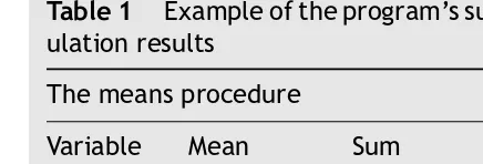
Table 1 Example of the program’s summation of sim-ulation results
The means procedure
Variable Mean Sum Std Error rejauc 0.9980000 998.0000000 0.0014135 rejcmax 1.0000000 1000.00 0
bothacc 0 0 0
h. simulated sampling times. 2. Treatment summary:
a. parameter correlation coefficients; b. computed parameter standard deviations; c. covariance matrix;
d. expected versus observed parameter means and standard deviations.
3. Output summary:
a. mean concentration versus time profiles, mean and standard deviation for AUC,Cmax, andTmax;
b. proc univariate output for all parameters and concentrations at each sampling time; c. schematic plots comparing treatment
popu-lation characteristics for the input parame-ters, drug concentrations at each sampling time, and bioavailability parameters; d. to facilitate the evaluation of the results over
a large number of replicates, the number of trials and proportion of the total number of replications that fail or succeed in meeting the bioequivalence criteria are summarized at the end of the simulation output. A sample output summary is featured isTable 1.
Under the column titled ‘‘Mean’’, this table pro-vides a synopsis of the fraction of the total number of replicates that failed to have confidence inter-vals contained within the bounds defining equiva-lence with respect to AUC (rejauc) andCmax( rejc-max). The proportion of simulated replicates when both AUC andCmax are contained within the bioe-quivalence criteria (bothacc) is also provided. The output also indicates the total number of replicates that fall within each of these categories (Sum), and the standard error about the mean ratio (Std Error).
4. Typical sample runs of the program
Identical seeds were used for all simulations in the following examples so that the output can be iden-tical except for changes specified by the coded pa-rameters.
4.1. One-compartment open body model
To demonstrate the data generation potential of this program, the various attributes are variants of the output generated with a one-compartmental open body model.
Model specifications
1. Subject per treatment = 24. 2. Number of replications = 1000. 3. Total dose = 100 mg.
4. Reference product parameter mean values:
Ka= 2 h−1; Vc= 1 L/kg; F= 0.50; Kel= 0.327 h−1. To demonstrate product inequivalence, the test product parameter values are Ka= 1.0 h−1 and
F= 0.35.
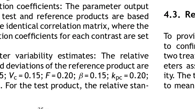
5. Correlation coefficients: The parameter output for the test and reference products will be based upon the identical correlation matrix, where the correlation coefficients for each contrast are set to 0.1. This minimizes the constraints about the resulting parameter values. Clearly, in some sit-uations (e.g., hepatic disease) there can be con-comitant changes in drug clearance (and there-foreKel) and volume of distribution as the con-centrations of serum albumin decrease[43]. Al-ternatively, there may be a relationship between
Ka and F, particularly if the drug is associated with a limited window of absorption within the small intestine. In these cases, F and Ka may be highly correlated[44]. Consequently, the in-vestigator needs to consider these physiological and pharmacokinetic properties when establish-ing the correlation coefficients.
6. Variability estimates: The relative standard de-viation of the reference product are as follow:
Ka= 0.25;Vc= 0.15; F= 0.20; Kel= 0.15. For the test product, the relative standard deviation are
Ka= 0.35;Vc= 0.15;F= 0.30;Kel= 0.15. Parame-ters are normally distributed.
7. Measurement error: Under the basic simula-tion condisimula-tions, there was no assay error, no pre-selected LOQ, and no subpopulations. Since the various dosing options have already been demonstrated, all other simulations were con-ducted as a single bolus administration.
The mean concentration/time profile for this simulation is shown inFig. 3.
4.2. Two-compartment open body model
Fig. 3 Mean and standard deviation of concentrations at each sampling time. Data are based upon a one-compartment open body model, using untransformed parameters, no assay noise and no specified lower limit of quantification.
Model specifications
1. Subject per treatment = 24. 2. Number of replications = 1000. 3. Total dose = 100 mg.
4. Reference product parameter mean values:
Ka= 2 h−1; Vc= 1 L/kg; F= 0.50; ˇ= 0.135 h−1;
kcp= 0.9 h−1; ˛= 2 h−1. To demonstrate product inequivalence, the test product parameter val-ues areKa= 1.0 h−1andF= 0.35.
5. Correlation coefficients: The parameter output for the test and reference products are based upon the identical correlation matrix, where the correlation coefficients for each contrast are set to 0.1.
6. Parameter variability estimates: The relative standard deviations of the reference product are
Ka= 0.25;Vc= 0.15;F= 0.20;ˇ= 0.15;kpc= 0.20;
˛= 0.20. For the test product, the relative
stan-dard deviations are identical to those of the reference product, except that Ka= 0.35 and
F= 0.30. All input parameters are normally dis-tributed.
7. Measurement error: All simulations are per-formed without any addition of analytical error.
The mean concentration versus time profiles generated under these simulation conditions are provided inFig. 4.
4.3. Relative bioavailability determinations
To provide an example of the program’s ability to confirm product comparability, we simulated two treatments containing pharmacokinetic param-eters associated with large intersubject variabil-ity. The two treatments were identical with respect to mean and variance values, and thus were truly
Table 2 Influence of subject number on bioequivalence determinations
Between-subject parameter values Ka(h−1) Vc (L/kg) F Kel(h−1)
(a) Simulation conditions for treatments 1 and 2 (one-compartment model)a
Treatments 1 and 2 2.0 (30%) 1.0 (15%) 0.50 (20%) 0.327 (15%)
#Subj/trt 10 15 20 24 30 40 100 1000
(b) Simulation output
Reject AUC 0.519 0.435 0.355 0.305 0.268 0.216 0.035 0 RejectCmax 0.398 0.315 0.236 0.206 0.173 0.117 0.11 0
Accept both 0.389 0.495 0.594 0.639 0.687 0.762 0.961 1.0
aResults if one considers the entire subject population. AUC 162g h/mL, 29% CV;C
max= 35 mg/mL, 26% CV; parameter values
for treatments 1 and 2 are identical.
equivalent. However, the ability to confirm equiva-lence under these conditions is generally limited by traditionally small number of observations included in these trials. Therefore, we modified the num-ber of subjects included per treatment, increas-ing study size from 10 to 1000. We conducted one thousand iterations of each run, and the propor-tion of successful runs where equivalence was con-firmed were assessed (Table 2). As expected, the power of the study to confirm bioequivalence in-creased as the number of subjects tended towards infinity.
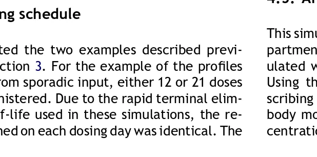
4.4. Dosing schedule
We simulated the two examples described previ-ously in Section3. For the example of the profiles resulting from sporadic input, either 12 or 21 doses were administered. Due to the rapid terminal elim-ination half-life used in these simulations, the re-sults obtained on each dosing day was identical. The
results of a 12 or 21 dose input schedule is provided over 2 dosing days inFig. 5.
We also simulated a random input schedule where the total dose is 100.0 mg and that this dose is administered once daily for three consecutive days or 33.3 mg per day. Each daily dose is ran-domly administered five times during the 24 h in-terval. The results of this simulation (simulated in four animals), using a one-compartment open body model with rapid input (Ka∼2 h−1) and elimination (T1/2∼2 h) is provided inFig. 6.
4.5. Analytical noise
This simulation is based upon the identical one com-partment body model previously described, sim-ulated without noise and without subpopulations. Using the pharmacokinetic parameter values de-scribing treatment 1 of the one-compartment open body model, the error about each simulated con-centration was defined by an 80% confidence that
Fig. 6 Simulation of four subjects receiving five random inputs over a 3-day dosing interval. Dose amount = 33 mg/day, T1/2∼2 h.
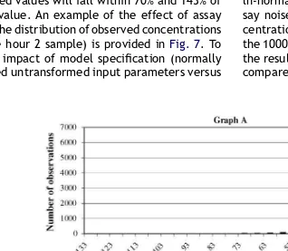
the assayed values will fall within 70% and 143% of the true value. An example of the effect of assay noise on the distribution of observed concentrations (e.g., the hour 2 sample) is provided inFig. 7. To show the impact of model specification (normally distributed untransformed input parameters versus
ln-normal distribution of input parameter) and as-say noise on the means and variances of the con-centrations at each sampling time (considered for the 1000 replications of 24 subjects per treatment), the resulting concentration versus time profiles are compared inTable 3(mean and CV for treatment 1).
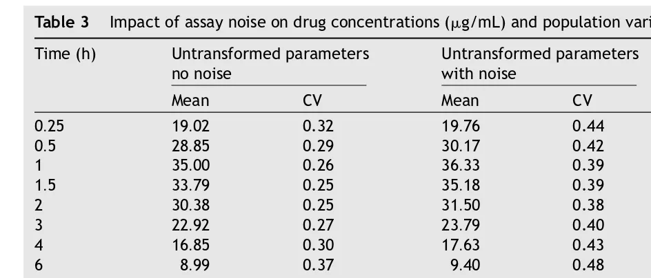
Table 3 Impact of assay noise on drug concentrations (g/mL) and population variance (expressed as %CV)
Time (h) Untransformed parameters no noise
Untransformed parameters with noise
ln-Transformed parameters no noise
Mean CV Mean CV Mean CV
0.25 19.02 0.32 19.76 0.44 19.00 0.32
0.5 28.85 0.29 30.17 0.42 28.85 0.29
1 35.00 0.26 36.33 0.39 35.00 0.26
1.5 33.79 0.25 35.18 0.39 33.79 0.25
2 30.38 0.25 31.50 0.38 30.38 0.25
3 22.92 0.27 23.79 0.40 22.92 0.27
4 16.85 0.30 17.63 0.43 16.85 0.30
6 8.99 0.37 9.40 0.48 8.99 0.37
8 4.82 0.46 5.00 0.55 4.82 0.46
12 1.42 0.66 1.48 0.74 1.42 0.65
16 0.43 0.90 0.45 0.98 0.43 0.91
24 0.05 1.51 0.05 1.57 0.05 1.51
36 0.0019 2.85 0.0020 3.00 0.0019 2.89
48 0.0001 4.77 0.0001 5.00 0.0001 5.00
4.6. Varying parameter constraints and
population characteristics
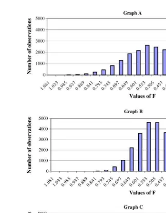
In most bioequivalence trials, it is F (the extent of product bioavailability) that is called into ques-tion. Therefore, we provide a frequency distribu-tion of the parameter output when it is simulated under the following conditions: a normal distribu-tion where the mean value is 0.95, the variability is characterized by a 20% CV, but values are not per-mitted to exceed 1.0 (Fig. 8); output based upon untransformed values but with a subpopulation pre-senting with a lower bioavailability (Fig. 9, Graph A); output based upon untransformed values but with a subpopulation presenting with the identical bioavailability as the main population (Fig. 9, Graph B);Fis generated on the basis of a single population (Fig. 9, Graph C). Not surprisingly, Graphs B and C are virtually identical.
4.7. AUC truncation
To illustrate the difference between the various truncated areas generated with this program, the basic treatment 2 AUC values (based upon the one-compartment model) is compared to those gener-ated whenloquant= 5 and (lowlim= 5,lowlimv= 1) (Table 4).
4.8. Distribution assumptions
To demonstrate the influence on parameter popula-tion distribupopula-tion on the resulting AUC values, AUC was generated under three simulation conditions: parametersKaandFwere simulated as if they were from a single normal distribution (Graph A); param-etersKaandFwere generated as if they were from a single ln-normal distribution (Graph B); andKaandF were simulated as if they were from two
Fig. 9 Comparison of the frequency distribution ofFvalues resulting from different population specifications: Graph A = 1000 replications of 24 subjects per treatment and the presence of a subpopulation where 30% of the population has a lower value ofF(F= 0.2) than does the primary population (F= 0.5). Graph B = 1000 replications of 24 subjects per treatment and the presence of a subpopulation, but in this case, the mean and variance estimates for these two populations are identical (F= 0.5). Graph C = 1000 replications of 24 subjects per treatment and a single population (F= 0.5). As would be expected, Graphs B and C are virtually identical.
ate normally distributions, where the main popula-tion had mean values of 0.35 and 1.0 h−1 forFand
Ka, respectively (%CV = 30% and 35% for Fand Ka, respectively), and 20% of the population had mean
values of 0.20 and 0.75 h−1 for F and K
a, respec-tively (%CV = 15% for both parameters). The basic set of pharmacokinetic parameters values used in this simulation procedure is identical to that
de-Table 4 Influence of designating different methods of lower limit cut-off values and different parameter distri-butions on the estimates of AUC0—48(mean and CV reflect values over the 1000 replications and 24 subjects per
treatment and replicate)
Untransformed parameters no noise
Untransformed parameters no noise loquant = 5
Untransformed parameters no noise lowlim = 5; lowlimv= 1
Mean 162.17 150.55 186.5
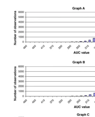
Fig. 10 Frequency distribution of AUC values resulting from the use of a one-compartment open body model with differing assumptions regarding the population distribution of the pharmacokinetic parameters. Graph A: parameters KaandFwere generated as a single normal distribution (F= 0.35, 30% CV;Ka= 1.0, 35% CV). Graph B: parametersKa
andFwere generated as a single ln-normal distribution based upon values described for Graph A. Graph C: parameter values forKa andFfollowed a multivariate normal distribution where 20% of the population were associated with
values forF= 0.20 (15% CV) andKa= 0.75 h−1(15% CV).
scribed for treatment 2, one-compartment open body model. The results of these simulations are provided inFig. 10.
5. Hardware/software specifications
This program was originally written for older ver-sions of SAS, but has been revised and tested on SAS version 8.2. We ran this version on a Pentium 300 MHz portable with 256 MB RAM. Bigger simula-tions may benefit from more RAM and more hard drive space. The user may want to customize the outputs using the Output Delivery System (ODS) that
now exists or modify various calculations provided within the program.
6. Mode of availability
pharmacologic and physiological conditions that can complicate the comparison of in vivo product performance.
An electronic copy of this program is available at no cost and can be downloaded from the University of Maryland website (www.biom.umd.edu).
Questions pertaining to the modeling attributes included in this program should be directed to M.N. Martinez [[email protected]]. Although the SAS coding generated by Dr. Russek-Cohen
Appendix A. Nomenclature
represents work completed while at the University of Maryland, Dr. Russek-Cohen currently is with the FDA. Therefore, questions pertaining to the coding used to translate these model considerations into a SAS program should be directed to E. Russek-Cohen at her current address at the Center for Devices and Radiation Health, Food and Drug Administration [[email protected]]. Questions pertaining to the handling of statistical concerns at CVM should be addressed to A.B. Nevius [[email protected]].
˛ distribution rate constant for the two-compartment body model (˛) amtdose vector with amount of drug given
AUC area under the concentration versus time curve
ˇ terminal elimination rate constant for a two-compartmental body model
corcoefr, corcoeft correlation of parameters within each group, reference and test. This must be a symmetric positive definite matrix. If two subpopulations per treatment (i.e., mix = 2) then same correlation matrix is used for each
cvref, cvtst coefficient of variation for each parameter, reference and test if mix = 2 then this is the CV for first subpopulation
cvref2, cvtst2 if mix = 2, then this is the CV for second subpopulation within each treatment Cmax the highest blood level concentration
confval tval×sqrt(1/n1 + 1/n2) where tval =t-value for 90% CI
d.f. degrees of freedom, ntot−2 =n1 +n2−2 fort-test for traditional bioequivalence test
dfrac totdose/nfractn implies amount in theith time period dosetim array with actual collection times
dosetype 1 = fixed schedule of dose inputs ndose is the number of doses
amtdose1, amtdose2 are arrays with amount of each bolus dose for reference and test dosetim1, dosetim2 are arrays with times of dose inputs for reference and test lasttime must be 1000 and is used to signal the end of an array
totdose1, totdose2 is the total drug input 2 = random schedule of dose inputs
nfractn is the number of dosing (time) intervals numimp is the number of dose inputs per interval ndose = nfractn×numimp (total number of dose inputs)
totdose is the total dose
lasttime is the last possible time for input drug
amtdose1, amtdose2, dosetim1, and dosetim2 are generated for each subject rather than for each treatment group
Default = 1
Kel elimination rate constant for a one-compartment body model
kpc intercompartmental rate constant, describing drug movement from the peripheral to central compartment
lasttime maximum time for the last dose
LOQ limit of quantification. Drug concentration values below the LOQ are deemed unreliable
loquant LOQ values
Default = 0.5
lowlim specified value at or below the LOQ for which all values falling below will be LOQ will be coded as the lowlimv. This will influence estimation of the AUC
Default = 0
lowlimv concentration value given to all data points below lowlim Default = 0
Lt lower limit to the 90% confidence bound. See comment in Section3.12
Mean rejauc proportion of times that the confidence bounds for the AUC fall outside the confi-dence limits set for confirming product bioequivalence and product bioequivalence is rejected
Mean rejcmax proportion of times that the confidence bounds for theCmaxfall outside the confi-dence limits set for confirming product bioequivalence and product bioequivalence is rejected
Mean bothacc proportion of time that the test and reference product meet the bioequivalence criteria for AUC andCmax
mncoeffr, mncoefft mean of parameters for reference and for test preparations
if mix = 2, then this is for first part of mixture. The program will use mncoefr2 and mncoeft2 for means of the second subpopulation within each treatment group. A binomial variable is used to determine number of subjects from each subpopulation
mncoefr2, mncoeft2 alternative mean vector for second subpopulation of each treatment group
measerr 0 = no measurement error will be added to the simulated drug concentrations 1 = a multiplicative measurement error is added to each simulated drug concentra-tion. . .additive on log scale of concentration
Default = 0
mix 1 = one population per treatment group
2 = two subpopulations for the specified pharmacokinetic variables
pmixf is the proportion of the population associated with the second less common population
ncompart 1 = one compartment model
npar = number of parameters = 4 (Ka,Vc,F,Kel) 2 = two compartment model
npar = number of parameters = 6 (Ka,kpc,Vc,˛,F,ˇ) Default = 1
nl,n2 sample sizes for reference (n1) and test (n2)
ndose number of doses
nfractn set tokimplies 1/kis proportion of total dose nmeas number of sample collection times
NREP number of datasets to be generated ntot n1 +n2 = total sample size
null 1 = test under situation where two groups are different 0 = test under situation where two groups are equal Default = 1
numimp number of doses in time 1/k
Outparm 1 = implies subject-specific parameters output with data anything else implies subject-specific parameters not output Default = 1
PARMTYPE 0 = single multivariate normal distribution within each treatment group 1 = single multivariate ln-normal population within each treatment group, where cv(y) = the coefficient of variation expressed on the linear scale;
v(y) = the variance of the untransformed data;
m(y) = the mean of the untransformed data;
v(x) = the variance of the ln-transformed data;
m(x) = the mean of the ln-transformed data;
cv(y′) = the coefficient of variation expressed on the linear scale based upon the back-transformed data
2 = mixture of two multivariate normal distributions within each treatment, where pmix1 = percent of population following the population parameter mean and vari-ability estimates
Default = 0
ptail specified when the user wishes to have values generated with ‘‘assay’’ error. For example, if we want the values generated with assay error to fall within 80—120% of the ‘‘true’’ values simulated without assay error, a ptail = 0.995 will generate noisy values such that we are 99% certain that these noisy values are within 80—120% of the value generated without assay noise. See Section3.6for exact usage
seed1, seed2 seeds for random number generators. It is recommended that the user specify a different seed for each treatment. If the same seed is repeated for sequential iter-ations, identical parameter values will be obtained. If seed is set to zero, the clock is used to generate a starting value for the random numbers. See SAS documentation on seed recommendations
stdcoefr, stdcoeft standard deviations of coefficients of reference and test groups. If mix = 2, then these represent standard deviations of first subpopulation within each treatment stdcofr2, stdckoft2 if mix = 2, these are the standard deviations for second subpopulation within each
treatment
tfrac lasttime/nfractn or time ofith time period
times collection times for blood plasma concentrations. These are assumed to be identical for both groups
timlbl actual blood plasma concentration collection times
Tmax the time at which the highest blood level concentration occurs totdose total dose over the course of a treatment
tval thet-value obtained from the student’st-distribution
Ut upper bound of the 90% confidence bound. See comment in Section3.12
References
[1] CVM guidance for industry: bioequivalence guidance, October 2002, http://www.fda.gov/cvm/guidance/ bioequivalence%Oct02.pdf(accessed date 11/03). [2] Center for Drug Evaluation and Research Guidance for
In-dustry: bioavailability and bioequivalence studies for orally administered drug products — general considerations, July 2002 (accessed date 11/03).
[3] D.Z. D’Argenio, D. Katz, Sampling strategies for noncom-partmental estimation of mean residence time, J. Pharma-cokin. Biopharm. 11 (1983) 435—446.
[4] M.S. Roberts, B.M. Magnusson, F.J. Burczynski, M. Weis, Enterohepatic circulation: physiological, pharmacokinetic and clinical implications, Clin. Pharmacokin. 4 (2002) 751—790.
[5] E. Lipka, I.D. Lee, P. Langguth, H. Spahn-Langguth, E. Mutschler, G.L. Amidon, Celiprolol double-peak occurrence and gastric motility: nonlinear mixed effects modeling of bioavailability data obtained in dogs, J. Pharmacokinet. Biopharm. 23 (1995) 267—286.
[6] Y. Wang, A. Roy, L. Sun, C.E. Lau, A double-peak phe-nomenon in the pharmacokinetics of alprazolam after oral administration, Drug Metab. Disp. 27 (1999) 855—859. [7] S.J. Veldhuyzen van Zanten, P.T. Pollak, H. Kapoor, P.K.
Ye-ung, Effect of omeprazole on movement of intravenously administered metronidazole into gastric juice and its sig-nificance in treatment of Helicobacter pylori, Dig. Dis. Sci. 41 (1996) 1845—1852.
[8] A.E. Pusateri, D.C. Kenison, Measurement of zeranol in plasma from three blood vessels in steers implanted with zeranol, J. Anim. Sci. 71 (1993) 415—429.
[9] D.M. Henricks, R.L. Edwards, K.A. Champe, T.W. Gettys, G.C. Skelly, T. Gimenez, Trenbolone, estradiol-17and es-trone levels in plasma and tissues and live weight gains of heifers implanted with trenbolone acetate, J. Anim. Sci. 55 (1982) 1048—1056.
[10] D.L. Zoran, D.H. Riedesel, D.C. Dyer, Pharmacokinetics of propofol in mixed-breed dogs and Greyhounds, Am. J. Vet. Res. 54 (1993) 755—760.
[11] M.H. Court, B.L. Hay-Kraus, D.W. Hill, A.J. Kind, D.L. Green-blatt, Propofol hydroxylation by dog liver microsomes; assay development and dog breed differences, Drug Metab. Disp. 27 (1999) 1293—1299.
[12] L.G. Lundin, M. Wilhelmson, Genetic variation of peptidase and pyrophosphatase in the chicken, Poultry Sci. 68 (1989) 1313—1318.
[13] J.C. Opdycke, R.E. Menzer, Pharmacokinetics of difluben-zuron in two types of chickens, J. Toxicol. Environ. Health. 13 (1984) 721—733.
[14] T.J. Danielson, W.G. Taylor, Pharmacokinetics of phenol-sulfonphthalein in sheep, Am. J. Vet. Res. 54 (1993) 2179—2183.
[15] B.O. Depelcin, S. Bloden, C. Michaux, M. Ansay, Effects of age, sex and breed on antipyrine disposition in calves, Res. Vet. Sci. 44 (1988) 135—139.
[16] C. Cristofol, M. Navarro, C. Franquelo, J.E. Valladares, M. Arboix, Sex differences in the disposition of albendazole metabolites in sheep, Vet. Parasit. 78 (1998) 223—231. [17] M. Oukessou, P.L. Toutain, Effect of dietary nitrogen intake
on gentamicin disposition in sheep, J. Vet. Pharmacol. Ther. 15 (1992) 416—420.
[18] Center for Drug Evaluation and Research Guidance For Industry: Statistical Approaches to Establishing Bioe-quivalence, posted 2/2001, http://www.fda.gov/cder/ guidance/3616fnl.pdf(accessed date 11/21/03).
[19] H. Ogata, N. Aoyagi, N. Kaniwa, M. Koibuchi, T. Shibazaki, A. Ejima, The bioavailability of diazepam from uncoated tablets in humans. Part II: Effect of gastric fluid acidity, Int. J. Clin. Pharmacol. Ther. Toxicol. 20 (1982) 166—170. [20] F.Y. Bois, T.N. Tozer, W.W. Hauck, M.L. Chen, R. Patnaik, R.L.
Williams, Bioequivalence: performance of several measures of extent of absorption, Pharm. Res. 11 (1994) 715—722. [21] F.Y. Bois, T.N. Tozer, W.W. Hauck, M.L. Chen, R. Patnaik, R.L.
Williams, Bioequivalence: performance of several measures of rate of absorption, Pharm. Res. 11 (1994) 966—974. [22] L. Endrenyi, F. Csizmadia, L. Tothfalusi, M.L. Chen,
Met-rics comparing simulated early concentration profiles for the determination of bioequivalence, Pharm. Res. 15 (1998) 1292—1299.
[23] L. Endrenyi, W. Yan, Variation of Cmax and Cmax/AUC in investigations of bioequivalence, Int. J. Clin. Pharmacol. Ther. Toxicol. 31 (1993) 184—189.
[24] K. Dhariwal, A. Jackson, Effect of length of sampling sched-ule and washout interval on magnitude of drug carryover from period 1 to period 2 in two-period, two-treatment bioequivalence studies and its attendant effects on deter-mination of bioequivalence, Biopharm. Drug Disp. 24 (2003) 219—228.
[25] J.L. Gabrielsson, DL. Weiner, Pharmacokinetic and Phar-macodynamic Data Analysis, Swedish Pharmaceutical Press, Stockholm, Sweden, 1997 (Chapter 3).
[26] R.N. Upton, Calculating the hybrid (macro) rate constants of a three-compartment mamillary pharmacokinetic model from known micro-rate constants, J. Pharmacol. Toxicol. Methods 49 (2004) 65—68.
[27] FDA Guidance for industry: FDA Approval of New Animal Drugs for Minor uses and For Minor Species (CVM Guidance #61), April 1999.
[28] M. Rowland, T.N. Tozer, R. Rowland, Clinical Pharmacoki-netics: Concepts and Applications, third ed., Lippincott, Williams & Wilkins, Philadeplphia, PA, 1995 (Chapter 19). [29] M. Weis, A novel extravascular input function for the
assess-ment of drug absorption in bioavailability studies, Pharm. Res. 13 (1996) 1547—1553.
[30] D.P. Schruimann, A comparison of the two one-sided tests procedure and the power approach for assessing the equiv-alence of average bioavailability, J. Pharm. Biopharm. 15 (1987) 657—680.
[31] P. Sathe, J. Venitz, L. Lesko, Evaluation of truncated areas in the assessment of bioequivalence of immediate release formulations of drugs with long half-lives and of Cmax with different dissolution rates, Pharm. Res. 16 (1999) 939—943. [32] L.F. Lacey, O.N. Keene, J.F. Pritchard, A. Bye, Common non-compartmental pharmacokinetic variables: are they nor-mally or ln-nornor-mally distributed, J. Biopharm. Stat. 7 (1997) 171—178.
[33] D.B. White, C.A. Walawander, D.Y. Liu, T.H. Grasela, Eval-uation of hypothesis testing for comparing two populations using NONMEM analysis, J. Pharmacokinet. Biopharm. 20 (1992) 295—313.
[34] D.B. White, C.A. Walawander, D.Y. Liu, T.H. Grasela, Re-buttal to the ‘‘letter to the editor’’ regarding ‘‘An eval-uation of point and interval estimates in population phar-macokinetics using NONMEM analysis’’, J. Pharmacokinet. Biopharm. 20 (1992) 393—395.
[35] E. Mizuta, A. Tsubotani, Preparation of mean drug concentration—time curves in plasma. A study on the fre-quency distribution of pharmacokinetic parameters, Chem. Pharm. Bull. 33 (1985) 1620—1632.
of population modeling, new ‘multiple model’ dosage de-sign, Bayesian feedback and individualized target goals, Clin. Pharmacokinet. 34 (1998) 55—77.
[37] E. Limbert, W.A. Stahel, M. Abbt, ln-Normal distributions across the sciences: keys and clues, BioScience 51 (2001) 341—352.
[38] Center for Drug Evaluation and Research and Center for Veterinary Medicine Guidance for Industry: bioanalytical method validation, May 2001,http://www.fda.gov/cder/ guidance/4252fnl.pdf(accessed date 12/10/03).
[39] R. Jellliffe, B. Tahani, Fitting drug concentration data according to its credibility: determining the assay er-ror pattern,http://www.lapk.org/pubsinfo/pdf/3-errs.pdf
(accessed date 12/10/03).
[40] M. de Hoog, R.C. Schoemaker, J.N. van den Anker, A.A. Vinks, NONMEM and NPEM2 population modeling: a
compar-ison using tobramycin data in neonates, Ther. Drug Monit. 24 (2002) 359—365.
[41] Y. Hyun, M. Ellis, F.K. McKeith, E.R. Wilson, Feed intake pat-tern of group-housed growing-finishing pigs monitored using a computerized feed intake recording system, J. Anim. Sci. 75 (1997) 1443—1451.
[42] J.A. Nienabe, T.P. McDonald, G.L. Hahn, Y.R. Chen, Eating dynamics of growing-finishing swine, Trans. ASAE 33 (1990) 2011—2018.
[43] J.F. Westphal, J.M. Brogard, Clinical pharmacokinetics of newer antibacterial agents in liver disease, Clin. Pharma-cokinet. 24 (1993) 46—58.