Variance Analysis of Linear SIMO Models with Spatially
Correlated Noise
⋆
Niklas Everitt
a, Giulio Bottegal
a, Cristian R. Rojas
a, H˚
akan Hjalmarsson
aa
ACCESS Linnaeus Center, School of Electrical Engineering, KTH - Royal Institute of Technology, Sweden
Abstract
Substantial improvement in accuracy of identified linear time-invariant single-input multi-output (SIMO) dynamical models is possible when the disturbances affecting the output measurements are spatially correlated. Using an orthogonal representation for the modules composing the SIMO structure, in this paper we show that the variance of a parameter estimate of a module is dependent on the model structure of the other modules, and the correlation structure of the disturbances. In addition, we quantify the variance-error for the parameter estimates for finite model orders, where the effect of noise correlation structure, model structure and signal spectra are visible. From these results, we derive the noise correlation structure under which the mentioned model parameterization gives the lowest variance, when one module is identified using less parameters than the other modules.
Key words: System identification, Asymptotic variance, Linear SIMO models, Least-squares.
1 Introduction
Recently, system identification in dynamic networks has gained popularity, see e.g., Van den Hof et al.(2013); Dankers et al. (2013b,a, 2014); Ali et al.(2011); Mat-erassiet al.(2011); Torreset al.(2014); Haber and Ver-haegen (2014); Gunes et al. (2014); Chiuso and Pil-lonetto (2012). In this framework, signals are modeled as nodes in a graph and edges model transfer functions. To estimate a transfer function in the network, a large number of methods have been proposed. Some have been shown to give consistent estimates, provided that a cer-tain subset of signals is included in the identification pro-cess (Dankerset al., 2013b,a). In these methods, the user has the freedom to include additional signals. However, little is known on how these signals should be chosen, and how large the potential is for variance reduction. From a theoretical point of view there are only a few re-sults regarding specific network structures e.g., H¨agget al.(2011); Ramaziet al.(2014); Wahlberget al.(2009). To get a better understanding of the potential of adding
⋆ This work was partially supported by the Swedish Re-search Council under contract 621-2009-4017, and by the Eu-ropean Research Council under the advanced grant LEARN, contract 267381.
Email addresses: [email protected](Niklas Everitt),
[email protected](Giulio Bottegal),[email protected](Cristian R. Rojas),[email protected](H˚akan Hjalmarsson).
available information to the identification process, we ask the fundamental questions: will, and how much, an added sensor improve the accuracy of an estimate of a certain target transfer function in the network? We shall attempt to give some answers by focusing on a special case of dynamic networks, namely single-input multi-output (SIMO) systems, and in a wider context, dynamic networks.
SIMO models are interesting in themselves. They find applications in various disciplines, such as signal pro-cessing and speech enhancement (Benestyet al., 2005), (Doclo and Moonen, 2002), communications (Bertaux
et al., 1999), (Schmidt, 1986), (Trudnowskiet al., 1998), biomedical sciences (McCombieet al., 2005) and struc-tural engineering (Ulusoyet al., 2011). Some of these ap-plications are concerned with spatio-temporal models, in the sense that the measured output can be strictly re-lated to the location at which the sensor is placed (Sto-icaet al., 1994), (Viberget al., 1997), (Viberg and Ot-tersten, 1991). In these cases, it is reasonable to expect that measurements collected at locations close to each other are affected by disturbances of the same nature. In other words, noise on the outputs can be correlated; un-derstanding how this noise correlation affects the accu-racy of the estimated model is a key issue in data-driven modeling of SIMO systems.
For SIMO systems, our aim in this contribution is to
quantify the model error induced by stochastic distur-bances and noise in prediction error identification. We consider the situation where the true system can accu-rately be described by the model, i.e., the true system lies within the set of models used, and thus the bias (systematic) error is zero. Then, the model error mainly consists of the variance-error, which is caused by distur-bances and noise when the model is estimated using a finite number of input-output samples. In particular, we shall quantify the variance error in terms of the noise covariance matrix, input spectrum and model structure. These quantities are also crucial in answering the ques-tions we have posed above, namely, when and how much, adding a sensor pays off in terms of accuracy of the es-timated target transfer function.
There are expressions for the model error, in terms of the asymptotic (in sample size) (co-) variance of the estimated parameters, for a variety of identification methods for multi-output systems (Ljung, 1999),(Ljung and Caines, 1980). Even though these expressions cor-respond to the Cram´er-Rao lower bound, they are typi-cally rather opaque, in that it is difficult to discern how the model accuracy is influenced by the aforementioned quantities. There is a well-known expression for the vari-ance of an estimated frequency response function that lends itself to the kind of analysis we wish to facilitate (Ljung, 1985; Yuan and Ljung, 1984; Zhu, 1989). This formula is given in its SIMO version by (see e.g., Zhu (2001))
Cov ˆG(ejω)≈ NnΦu(ω)−1Φv(ω), (1)
whereΦuis the input spectrum andΦvis the spectrum
of the noise affecting the outputs. Notice that the ex-pression is valid for large number of samples N and large model order n. For finite model order there are mainly results for SISO models (Hjalmarsson and Nin-ness, 2006; Ninness and Hjalmarsson, 2004, 2005a,b) and recently, multi-input-single-output (MISO) models. For MISO models, the concept of connectedness (Gev-erset al., 2006) gives conditions on when one input can help reduce the variance of an identified transfer func-tion. These results were refined in M˚artensson (2007). For white inputs, it was recently shown in Ramazi et al. (2014) that an increment in the model order of one transfer function leads to an increment in the variance of another estimated transfer function only up to a point, after which the variance levels off. It was also quan-tified how correlation between the inputs may reduce the accuracy. The results presented here are similar in nature to those in Ramazi et al. (2014), while they regard another special type of multi-variable models, namely multi-input single-output (MISO) models. Note that variance expressions for the special case of SIMO cascade structures are found in Wahlberg et al.(2009), Everittet al.(2013).
1.1 Contribution of this paper
As a motivation, let us first introduce the following two output example. Consider the model:
y1(t) =θ1,1u(t−1) +e1(t), y2(t) =θ2,2u(t−2) +e2(t),
where the input u(t) is white noise and ek, k = 1,2 is
measurement noise. We consider two different types of measurement noise (uncorrelated with the input). In the first case, the noise is perfectly correlated, let us for sim-plicity assume thate1(t) = e2(t). For the second case, e1(t) ande2(t) are independent. It turns out that in the first case we can perfectly recover the parametersθ1,1 andθ2,2, while, in the second case we do not improve the
accuracy of the estimate ofθ1,1 by also using the mea-surementy2(t). The reason for this difference is that, in the first case, we can construct the noise free equation
y1(t)−y2(t) =θ1,1u(t−1)−θ2,2u(t−2) and we can perfectly recoverθ1,1 andθ2,2, while in the
second case neithery2(t) nore2(t) contain information aboute1(t).
Also the model structure plays an important role for the benefit of the second sensor. To this end, we consider a third case, where again e1(t) =e2(t). This time, the model structure is slightly different:
y1(t) =θ1,1u(t−1) +e1(t), y2(t) =θ2,1u(t−1) +e2(t).
In this case, we can construct the noise free equation
y1(t)−y2(t) = (θ1,1−θ2,2)u(t−1).
The fundamental difference is that now only the differ-ence (θ1,1−θ2,1) can be recovered exactly, but not the
parametersθ1,1andθ2,1themselves. They can be identi-fied fromy1(t) andy2(t) separately, as long asy1andy2 are measured. A similar consideration is made in Ljung
et al. (2011), where SIMO cascade systems are consid-ered.
This paper will generalize these observations in the fol-lowing contributions:
• For a non-white input spectrum, we show where in the frequency spectrum the benefit of the correla-tion structure is focused.
• When one module, i.e., the relationship between the input and one of the outputs, is identified using less parameters, we derive the noise correlation struc-ture under which the mentioned model parameter-ization gives the lowest total variance.
The paper is organized as follows: in Section 2 we define the SIMO model structure under study and provide an expression for the covariance matrix of the parameter estimates. Section 3 contains the main results, namely a novel variance expression for LTI SIMO orthonormal basis function models. The connection with MISO mod-els is explored in Section 4. In Section 5, the main results are applied to a non–white input spectrum. In section 6 we derive the correlation structure that gives the mini-mum total variance, when one block has less parameters than the other blocks. Numerical experiments illustrat-ing the application of the derived results are presented in Section 7. A final discussion ends the paper in Section 8.
2 Problem Statement
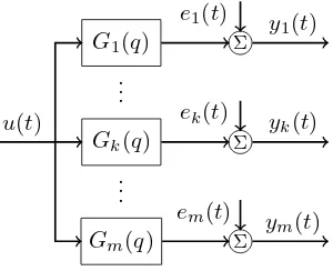
Fig. 1.Block scheme of the linear SIMO system.
We consider linear time-invariant dynamic systems with one input andmoutputs (see Fig. 1). The model is de-scribed as follows:
whereqdenotes the forward shift operator, i.e.,qu(t) = u(t+ 1) and theGi(q) are causal stable rational transfer
functions. TheGiare modeled as
Gi(q, θi) =Γi(q)θi, θi ∈Rni, i= 1, . . . , m, (3) thonormal with respect to the scalar product defined for complex functions f(z), g(z) : C → C1×m as hf, gi := white, but may be correlated in the spatial domain:
E [e(t)] = 0 Ee(t)e(s)T=δ
t−sΛ (4)
for some positive definite matrix covariance matrix Λ, and where E [·] is the expected value operator. We ex-pressΛin terms of its Cholesky factorization
Λ=ΛCHΛTCH, (5) We summarize the assumptions on input, noise and model as follows:
Assumption 1 The input{u(t)} is zero mean station-ary white noise with finite moments of all orders, and varianceσ2>0. The noise{e(t)}is zero mean and
tem-porally white, i.e,(4) holds withΛ > 0, a positive def-inite matrix. It is assumed that E|e(t)|4+ρ < ∞ for
someρ >0. The data is generated in open loop, that is, the input{u(t)}is independent of the noise{e(t)}. The true input-output behavior of the data generating system can be captured by our model, i.e the true system can be described by (2)and (3)for some parametersθo
i ∈Rni,
i = 1, . . . , m, where n1 ≤. . . ≤ nm. The orthonormal
basis functions{Bk(q)}are assumed stable. ✷
• The assumption that the modules have the same or-thogonal parameterization in (3) is less restrictive than it might appear at first glance, and made for clarity and ease of presentation. A model consist-ing of non-orthonormal basis functions can be trans-formed into this format by a linear transformation, which can be computed by the Gram-Schmidt proce-dure (Trefethen and Bau, 1997). Notice that fixed denominator models, with the same denominator in all transfer functions, also fit this framework (Nin-ness et al., 1999). However, it is essential for our analysis that the modules share poles.
• It is not necessary to restrict the input to be white noise. A colored input introduces a weight-ing by its spectrum Φu, which means that the
basis functions need to be orthogonal with re-spect to the inner product hf, giΦu := hf Φu, gi.
If Φu(z) = σ2R(z)R∗(z), where R(z) is a monic
stable minimum phase spectral factor; the trans-formation Γ˜i(q) = σ−1R(q)−1Γi(q) is a procedure
that gives a set of orthogonal basis functions in the weighted space. If we use this parameterization, all the main results of the paper carry over naturally. However, in general, the new parameterization does not contain the same set of models as the original parameterization. Another way is to use the Gram-Schmidt method, which maintains the same model set and the main results are still valid. If we would like to keep the original parameterization, we may, in some cases, proceed as in Section 5 where the input signal is generated by an AR-spectrum.
• Note that the assumption thatn1≤. . .≤nmis not
restrictive as it only represents an ordering of the modules in the system.
2.1 Weighted least-squares estimate
By introducing θ=hθT
1, . . . , θTm iT
∈Rn,n:=Pmi=1ni
and then×mtransfer function matrix
˜ Ψ(q) =
Γ1 0 0 0 . .. 0
0 0 Γm
,
we can write the model (2) as a linear regression model
y(t) =ϕT(t)θ+e(t), (8)
where
ϕT(t) = ˜Ψ(q)Tu(t).
An unbiased and consistent estimate of the parameter vector θ can be obtained from weighted least-squares, with optimal weighting matrix Λ−1 (see, e.g., Ljung
(1999); S¨oderstr¨om and Stoica (1989)). Λ is assumed known, however, this assumption is not restrictive since Λcan be estimated from data. The estimate ofθis given by
ˆ θN =
N X
t=1
ϕ(t)Λ−1ϕT(t)
!−1
N X
t=1
ϕ(t)Λ−1y(t). (9)
Inserting (8) in (9) gives
ˆ
θN = θ+ N X
t=1
ϕ(t)Λ−1ϕT(t)
!−1
N X
t=1
ϕ(t)Λ−1e(t).
Under Assumption 1, the noise sequence is zero mean, hence ˆθN is unbiased. It can be noted that this is the
same estimate as the one obtained by the prediction er-ror method and, if the noise is Gaussian, by the max-imum likelihood method (Ljung, 1999). It also follows that the asymptotic covariance matrix of the parameter estimates is given by
AsCov ˆθN = E
ϕ(t)Λ−1ϕT(t)−1. (10)
Here AsCov ˆθN is the asymptotic covariance matrix
of the parameter estimates, in the sense that the asymptotic covariance matrix of a stochastic sequence {fN}∞N=1, fN ∈C1×q is defined as1
AsCovfN := lim
N→∞N·E [(fN −E [fN]) ∗(f
N −E [fN])].
In the problem we consider, using Parseval’s formula and (7), the asymptotic covariance matrix, (10), can be written as2
AsCov ˆθN =
1 2π
Z π
−π
Ψ(ejω)Ψ∗(ejω) dω −1
=hΨ, Ψi−1, (11)
where
Ψ(q) = 1 σΨ˜(q)Λ
−T
CH. (12)
Note that Ψ(q) is block upper triangular since ˜Ψ(q) is block diagonal andΛ−CHT is upper triangular.
1
This definition is slightly non-standard in that the second term is usually conjugated. For the standard definition, in general, all results have to be transposed, however, all results in this paper are symmetric.
2
2.2 The introductory example
With formal assumptions in place, we now consider the introductory example in greater detail. Consider the model
y1(t) =θ1,1q−1u(t) +e1(t), (13) y2(t) =θ2,1q−1u(t) +θ2,2q−2u(t) +e2(t) (14) which uses the delaysq−1andq−2as orthonormal basis functions. With θ = [θ1,1θ2,1θ2,2]T; the corresponding
regression matrix is
ϕ(t)T = "
u(t−1) 0 0
0 u(t−1) u(t−2)
#
.
The noise vector is generated by
"
e1(t) e2(t)
#
=Lw(t) =
"
1 0
p
1−β2 β
# "
w1(t) w2(t)
#
, (15)
wherew1(t) andw2(t) are uncorrelated white processes with unit variance. The parameterβ ∈[0,1] tunes the correlation betweene1(t) ande2(t). Whenβ= 0, the two processes are perfectly correlated (i.e., identical); con-versely, whenβ = 1, they are completely uncorrelated. Note that, for every β ∈ [0, 1], one has Ee1(t)2 = Ee2(t)2= 1. In fact, the covariance matrix ofe(t) be-comes
Λ=LLT = "
1 p1−β2
p
1−β2 1
#
.
Then, when computing (11) in this specific case gives
AsCov ˆθN =
1 σ2
1 p1−β2 0
p
1−β2 1 0
0 0 β2
. (16)
We note that:
AsCov hθˆ1,1 θˆ2,1iT = 1 σ2Λ, AsCov ˆθ2,2=
1 σ2β
2.
The above expressions reveals two interesting facts:
(1) The (scalar) variances of ˆθ1,1 and ˆθ2,1, namely the
estimates of parameters of the two modules related to the same time lag, are not affected by possible
correlation of the noise processes, i.e., they are in-dependent of the value ofβ. However, note that the cross correlation between ˆθ1,1and ˆθ2,1in (16):
Var (ˆθ1,1−
p
1−β2θˆ 2,1)
=
"
1 −p1−β2
#T
1 σ2Λ
"
1 −p1−β2
#
= 1 σ2β
2. (17)
This cross correlation will induce a cross correlation in the transfer function estimates as well.
(2) As seen in (16), the variance of ˆθ1,2 strongly de-pends onβ. In particular, whenβ tends to 0, one is ideally able to estimate ˆθ1,2 perfectly. Note that in the limit case β = 0 one hase1(t) = e2(t), so that (2) can be rearranged to obtain the noise-free equation
y1(t)−y2(t) = (θ1,1−θ2,1)u(t−1) +θ1,2u(t−2), which shows that bothθ1,2and the differenceθ1,1− θ2,1 can be estimated perfectly. This can of course also be seen from (16), cf. (17).
The example shows that correlated measurements can be favorable for estimating for estimating certain pa-rameters, but not necessarily for all. The main focus of this article is to generalize these observations to arbi-trary basis functions, number of systems and number of estimated parameters. Additionally, the results are used to derive the optimal correlation structure of the noise. But first, we need some technical preliminaries.
2.3 Review of the geometry of the asymptotic variance
The following lemma is instrumental in deriving the re-sults that follow.
Lemma 3 (Lemma II.9in Hjalmarsson and M˚artensson (2011)) LetJ :Rn→C1×q be differentiable with respect
to θ, and Ψ ∈ Ln×m
2 ; let SΨ be the subspace of L1×m
spanned by the rows ofΨ and{BS
k}rk=1, r≤nbe an
or-thonormal basis for SΨ. Suppose that J′(θo) ∈Cn×q is
the gradient ofJ with respect toθandJ′(θo) =Ψ(z o)L
for somez0∈CandL∈Cm×q. Then
AsCovJ(ˆθN) =L∗ r X
k=1
BkS(zo)∗BSk(zo)L. (18)
2.4 Non-estimable part of the noise
variance error will depend on the non-estimable part of the noise, i.e., the part that cannot be linearly estimated from other noise sources. To be more specific, define the signal vector ej\i(t) to include the noise sources from
module 1 to modulej, with the one from modulei ex-cluded, i.e.,
ej\i(t) :=
h
e1(t), . . . , ej(t) iT
j < i,
h
e1(t), . . . , ei−1(t) iT
j=i,
h
e1(t), . . . , ei−1(t), ei+1(t), . . . , ej(t) iT
j > i.
Now, the linear minimum variance estimate ofei given
ej\i(t), is given by
ˆ
ei|j(t) :=̺ijTej\i(t). (19)
Introduce the notation
λi|j:= Var [ei(t)−eˆi|j(t)], (20)
with the convention that λi|0 := λi. The vector ̺ij in
(19) is given by
̺ij =
Covej\i(t) −1
Eej\i(t)ei(t)
. We call
ei(t)−eˆi|j(t)
the non-estimable part ofei(t) givenej\i(t).
Definition 4 When ˆei|j(t) does not depend on ek(t),
where1 ≤k≤j,k =6 i, we say thatei(t)is orthogonal
toek(t)conditionally toej\i(t).
The variance of the non-estimable part of the noise is closely related to the Cholesky factor of the covariance matrixΛ. We have the following lemma.
Lemma 5 Let e(t) ∈ Rm have zero mean and
covari-ance matrix Λ > 0. Let ΛCH be the lower triangular
Cholesky factor ofΛ, i.e.,ΛCH satisfies(5), with{γik}
as its entries as defined by (6). Then forj < i,
λi|j= i X
k=j+1 γ2ik.
Furthermore,γij = 0is equivalent to thatei(t) is
orthog-onal toej(t) conditionally toej\i(t).
PROOF. See Appendix A.
Similar to the above, fori≤m, we also define
ei:m(t) := h
ei(t) . . . em(t) iT
,
and forj < iwe define ˆei:m|j(t) as the linear minimum
variance estimate ofei:m(t) based on the other signals
ej\i(t), and
Λi:m|j := Cov [ei:m(t)−eˆi:m|j(t)].
As a small example of why this formulation is useful, consider the covariance matrix below, where there is cor-relation between any pair (ei(t), ej(t)):
Λ=
1 0.6 0.9 0.6 1 0.54 0.9 0.54 1
=
1 0 0
0.6 0.8 0 0.9 0 0.44
| {z }
ΛCH
1 0.6 0.9 0 0.8 0 0 0 0.44
.
From the Cholesky factorization above we see that, since γ32 is zero, Lemma 5 gives that e3(t) is orthogonal to e2(t) given e2\3(t), i.e., there is no information about e3(t) ine2(t) if we already knowe1(t). This is not ap-parent fromΛwhere every entry is non-zero. If we know e1(t) a considerable part ofe2(t) ande3(t) can be esti-mated. Without knowinge1(t),λ1=λ2=λ3= 1, while if we knowe1(t),λ2|1= 0.64 andλ3|1= 0.19.
3 Main results
In this section, we present novel expressions for the variance-error of an estimated frequency response func-tion. The expression reveals how the noise correlation structure, model orders and input variance affect the variance-error of the estimated frequency response func-tion. We will analyze the effect of the correlation struc-ture of the noise on the transfer function estimates. To this end, collect allmtransfer functions into
G:=hG1 G2 . . . Gm i
.
For convenience, we will simplify notation according to the following definition:
Definition 6 The asymptotic covariance ofGˆ(ejω0) := G(ejω0,θˆN)for the fixed frequencyω
0is denoted by
AsCov ˆG.
In particular, the variance ofGˆi(ejω0) := Gi(ejω0,θˆiN)
Defineχkas the index of the first system that contains the
basis functionBk(ejω0). Notice thatχk−1is the number
of systems that do not contain the basis function.
Theorem 7 Let Assumption 1 hold. Suppose that the parameters θi ∈Rni,i= 1, . . . , m, are estimated using
weighted least-squares(9). Let the entries ofθbe arranged as follows:
¯
θ= [θ1,1 . . . θm,1 θ1,2 . . . θm,2. . . θ1,n1 . . . . . . θm,n1θ2,n1+1 . . . θm,n1+1 . . . θm,nm]
T.(21)
and the corresponding weighted least-squares estimate be denoted byθˆ¯. Then, the covariance ofθˆ¯is
AsCov ˆθ¯= 1
σ2diag(Λ1:m, Λχ2:m|χ2−1, . . . ,
. . . , Λχnm:m|χnm−1). (22)
In particular, the covariance of the parameters related to basis function numberkis given by
AsCov ˆθ¯k=
1
σ2Λχk:m|χk−1, (23)
where
ˆ¯ θk=
h
ˆ
θχk,k . . .θˆm,k
iT
,
and where, forχk≤i≤m,
AsVar ˆθi,k=
λi|χk−1
σ2 . (24)
It also holds that
AsCov ˆG=
nm
X
k=1
"
0χk−1 0
0 AsCov ˆ¯θk #
|Bk(ejω0)|2, (25)
where AsCov ˆ¯θk is given by (23) and0χk−1 is a χk − 1 ×χk −1 matrix with all entries equal to zero. For
χk = 1, 0χk−1 is an empty matrix. In (25),0 denotes
zero matrices of dimensions compatible to the diagonal blocks.
PROOF. See Appendix B.
Remark 8 The covariance ofθˆ¯k, which contain the
pa-rameters related to basis function k, is determined by which other models share the basis functionBk; cf. (17)
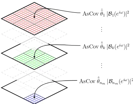
of the introductory example. The asymptotic covariance ofGˆcan be understood as a sum of the contributions from each of thenmbasis functions. The covariance
contribu-tion from a basis funccontribu-tionBk is weighted by |Bk(ejω0)|2
and only affects the covariance between systems that con-tain that basis function, as visualized in Figure 2.
AsCov ˆ˜θ
1|B1(eiω)|2
AsCov ˆ˜θk|Bk(eiω)|2
AsCov ˆ˜θn
m|Bnm(e
iω
)|2 ...
...
Fig. 2. A graphical representation of AsCov ˆGwhere each term of the sum in (25) is represented by a layer. A basis function only affects the covariance between modules that also contain that basis function. Thus, the first basis function affects the complete covariance matrix while the last basis functionnmonly affects modulesχnm, . . . , m.
Remark 9 The orthogonal basis functions correspond to a decomposition of the output signals into orthogonal components and the problem in a sense becomes decou-pled. As an example, consider the system described by
y1(t) =θ1,1B1(q)u(t) +e1(t), y2(t) =θ2,1B1(q)u(t) +e2(t),
y3(t) =θ3,1B1(q)u(t) +θ3,2B2(q)u(t) +e3(t), (26)
Suppose that we are interested in estimatingθ3,2. For this
parameter,(24)becomes
AsVar ˆθ3,2= λ3|2
σ2 (27)
To understand the mechanisms behind this expression, let u1(t) = B1(q)u(t), and u2(t) = B2(q)u(t) so that the system can be visualized as in Figure 3, i.e., we can consideru1andu2as separate inputs.
First we observe that it is onlyy3that contains
informa-tion aboutθ3,2, and the termθ3,1u1contributing toy3is
a nuisance from the perspective of estimatingθ3,2. This
term vanishes when u1 = 0and we will not be able to
achieve better accuracy than the optimal estimate ofθ3,2
for this idealized case. So let us study this setting first. Straightforward application of the least-squares method, usingu2 andy3, gives an estimate ofθ3,2with variance λ/σ2, which is larger than (27)whene3 depends one1
and e2. However, in this idealized case, y1 = e1 and y2 = e2, and these signals can thus be used to estimate e3. This estimate can then be subtracted fromy3 before
the least-squares method is applied. The remaining noise iny3will have varianceλ3|2, ife3is optimally estimated
To understand why it is possible to achieve the same ac-curacy as this idealized case when u1 is non-zero, we
need to observe that our new inputs u1(t)andu2(t)are orthogonal (uncorrelated)3. Returning to the case when
only the outputy3is used for estimatingθ3,2, this implies
that we pay no price for including the termθ3,1u1in our
model, and then estimatingθ3,1andθ3,2jointly, i.e., the
variance ofθˆ3,2will still beλ/σ2 4. The question now is
if we can usey1andy2as before to estimatee3. Perhaps
surprisingly, we can use the same estimate as when u1
was zero. The reader may object that this estimate will now, in addition to the previous optimal estimate ofe3,
contain a term which is a multiple ofu1. However, due
to the orthogonality between u1 and u2, this term will
only affect the estimate of θ3,1 (which we anyway were
not interested in, in this example), and the accuracy of the estimate of θ3,2 will beλ3|2/σ2, i.e. (27). Figure 4
illustrates the setting with y˜3 denoting y3 subtracted by
the optimal estimate ofe3. In the figure, the new
param-eter θ˜3,1 reflects that the relation between u1 and y˜3 is
different fromθ3,1as discussed above. A key insight from
this discussion is that for the estimate of a parameter in the path from inputito outputj, it is only outputs that are not affected by input ithat can be used to estimate the noise in output j; when this particular parameter is estimated, using outputs influenced by inputiwill intro-duce a bias, since the noise estimate will then contain a term that is not orthogonal to this input. In (24), this manifests itself in that the numerator isλi|χk−1, only the χk−1first systems do not containui.
θ1,1 Σ
e1(t) y1(t)
u1(t)
θ2,1 Σ
e2(t) y2(t)
θ3,1 Σ
e3(t) y3(t)
u2(t)
θ3,2
Fig. 3. The SIMO system of Remark 9, described by (26).
We now turn our attention to the variance of the indi-vidual transfer function estimates.
3
This sinceu(t) is white andB1andB2 are orthonormal. 4
Withu1andu2correlated, the variance will be higher, see
Section 4 for a further discussion of this topic.
θ1,1 Σ
e1(t)
y1(t)
u1(t)
θ2,1 Σ
e2(t)
y2(t)
u1(t) ˜
θ3,1 Σ
e3(t)−e3|2ˆ (t) ˜
y3(t)
u2(t)
θ3,2
Fig. 4. The SIMO system of Remark 9, described by (26), but with ˜y3denotingy3subtracted by the optimal estimate
ofe3and ˜θ3,1reflects that the relation betweenu1 and ˜y3is
different fromθ3,1.
Corollary 10 Let the same assumptions as in Theo-rem 7 hold. Then, for any frequencyω0, it holds that
AsVar ˆGi= ni
X
k=1
|Bk(ejω0)|2AsVar ˆθi,k, (28)
where
AsVar ˆθi,k=
λi|χk−1
σ2 , (29)
andλi|jis defined in (20).
PROOF. Follows from Theorem 7, since (28) is a
di-agonal element of (25).
From Corollary 10, we can tell when increasing the model order ofGj will increase the asymptotic variance of ˆGi.
Corollary 11 Under the same conditions as in Theo-rem 7, if we increase the number of estimated parameters ofGjfromnjtonj+1, the asymptotic variance ofGiwill
increase, if and only if all the following conditions hold:
(1) nj< ni,
(2) ei(t) is not orthogonal to ej(t) conditioned on
ej\i(t),
(3) |Bnj+1(e
jω0)|26= 0.
Remark 12 Corollary 11 explicitly tells when an in-crease in the model order of Gj from nj tonj+ 1 will
increase the variance of Gi. Ifnj ≥ni, there will be no
increase in the variance ofGi, no matter how many
ad-ditional parameters we introduce to the modelGj, which
was also seen the introductory example in Section 2.2. Naturally, if ei(t)is orthogonal to ej(t)conditioned on
ej\i(t),eˆi|j(t) does not depend onej(t) and there is no
increase in variance ofGˆi, cf. Remark 9.
3.1 A graphical representation of Corollary 11
Following the notation in Bayesian Networks (Koski and Noble, 2012), Conditions 1) and 2) in Corollary 11 can be interpreted graphically. Each module is represented by a vertex in a weighted directed acyclic graph G. Let the vertices be ordered by model order, i.e., let the first vertex correspond to ˆG1. Under Assumption 1, with the additional assumption that moduleiis the first module with orderni, let there be an edge, denoted by j → i,
from vertexjtoi,j < i, ifei(t) is not orthogonal toej(t)
conditioned on ej\i(t). Notice that this is equivalent to
γij 6= 0. Let the weight of the edge beγij and define
the parents of vertex i to be all nodes with a link to vertexi, i.e.,paG(i) :={j:j→i}. Then, (29), together with Lemma 5, shows that only outputs corresponding to parents of nodeiaffect the asymptotic variance. Indeed, a vertex without parents has variance
AsVar ˆGi=
which corresponds to (28) with
λi|0=. . .=λi|i−1=λi.
Thus, AsVar ˆGiis independent of the model order of the
other modules.
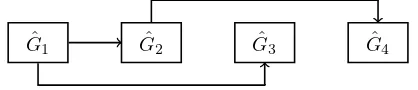
As an example, consider four systems with the lower Cholesky factor of the covariance ofe(t) given by:
Λ=
If the model orders are distinct, the corresponding graph is given in Figure 5, where one can see that AsVar ˆG4 depends ony2(and ony4of course), but depends neither ony3nory1sinceγ43=γ41= 0, AsVar ˆG3depends on y1, but not ony2sinceγ32= 0 and AsVar ˆG2depends on y1, while the variance of ˆG1is given by (30). Ifn2=n4, the first condition of Corollary 11 is not satisfied and we have to cut the edge between ˆG4 and ˆG2. Similarly, if
Fig. 5. Graphical representation of Conditions 1) and 2) in Corollary 11 for the Cholesky factor given in (31).
4 Connection between MISO and SIMO
There is a strong connection between the results pre-sented here and those regarding MISO systems prepre-sented in Ramaziet al.(2014). We briefly restate the problem formulation and some results from Ramaziet al.(2014) to show the connection. The MISO data generating sys-tem is in some sense the dual of the SIMO case. With m spatially correlated inputs and one output, a MISO system is described by
y(t) =hG1(q) G2(q) . . . Gm(q) white, but may be correlated in the spatial domain,
E [u(t)] = 0 Eu(t)u(s)T=δt−sΣu,
for some positive definite matrix covariance matrixΣu=
ΣCHΣCHT , whereΣCH is the lower triangular Cholesky
factor ofΣ. The noisee(t) is zero mean and has variance λ. The asymptotic covariance of the estimated parame-ters can be expressed using (11) with
Ψ =ΨMISO:= ˜Ψ Σ
CH. (32)
We make the convention that Pk2
Theorem 13 (Theorem 4 in Ramaziet al.(2014))
Under Assumption 1, but withn1≥n2≥. . . ,≥nm, for
any frequencyω0it holds that
AsVar ˆGi= m X
j=i
λ σ2
i|j nj
X
k=nj+1+1
|Bk(ejω0)|2, (33)
where nm+1 := 0 and σ2i|j is the variance of the
non-estimable part ofui(t)givenuj\i(t).
Corollary 14 (Corollary 6 in Ramaziet al.(2014))
Under Assumption 1, but with n1 ≥ n2 ≥ . . . ,≥ nm.
Suppose that the order of blockjis increased fromnj to
nj+1. Then there is an increase in the asymptotic
vari-ance ofGˆiif and only if all the following conditions hold:
(1) nj< ni,
(2) ui(t) is not orthogonal to uj(t) conditioned on
uj\i(t),
(3) |Bnj+1(e
jω0)|26= 0.
Remark 15 The similarities between Corollary 10 and Theorem 13, and between Corollary 11 and Corollary 14 are striking. In both cases it is the non-estimable part of the input and noise, respectively, along with the estimated basis functions that are the key determinants for the re-sulting accuracy. Just as in Corollary 10, Theorem 13 can be expressed with respect to the basis functions:
AsVar ˆGi= ni
X
k=1
AsVar ˆθi,k|Bk(ejω0)|2. (34)
However, now
AsVar ˆθi,k=
λ σ2
i|χk
(35)
whereσ2
i|lis determined by the correlation structure of the
inputsui(t)to the systemsGi(q, θi)that doshare basis
function Bk(q)(i = 1, . . . , χk). Note that in the SIMO
case we had
AsVar ˆθi,k =
λi|χk σ2
whereλi|χkis determined by the correlation structure of
the noise sources ei(t) affecting systems Gi(q, θi) that
do not share basis functionBk(q)(i = 1, . . . , χk). Note
that (33)found in Ramazi et al. (2014) does not draw the connection to the variance of the parameters. This is made explicit in the alternate expressions(35)and(34).
The correlation between parameters related to the same basis functions is not explored in Ramaziet al.(2014). In fact, it is possible to follow the same line of reasoning leading to Theorem 7 and arrive at the counter-part for
MISO systems. Let the first χk systems contain basis
functionk, so
AsVar ˆθ¯kM ISO=λ Σ1:−1χk
where Σ1:χk denotes the covariance matrix of the first χk inputs. Hence
AsCov ˆG=λ
n1
X
k=1
"
Σ1:−1χk 0 0 0m−χk
#
|Bk(ejω0)|2,
and
AsCov ˆθ¯M ISO=λ diag(Σ−1 1:χ1, Σ
−1
1:χ2, . . . , Σ −1
1:χnm).(36) Note that, while the correlation between the noise sources is beneficial, the correlation in the input is detri-mental for the estimation accuracy. Intuitively, if we use the same input to parallel systems, and only observe the sum of the outputs, there is no way to determine the contribution from the individual systems. On the other hand, as observed in the example in Section 2.2, if the noise is correlated, we can construct equations with re-duced noise and improve the accuracy of our estimates.
This difference may also be understood from the struc-ture of Ψ, which through (11) determines the variance properties of any estimate. Consider a single SISO sys-temG1as the basic case. For the SIMO structure con-sidered in this paper, as noted before,ΨSIMOof (12) is block upper triangular withmcolumns (the number of outputs), whileΨMISOis block lower triangular with as many columns as inputs.ΨMISOis block lower triangu-lar since ˜Ψ is block diagonal andΣCH is lower
triangu-lar in (32). Adding an outputyj to the SIMO structure
corresponds to extendingΨSIMO with one column (and nj rows):
ΨeSIMO= "
ΨSIMO ⋆
0 ⋆
#
, (37)
where the zero comes from thatΨSIMO
e also is block
up-per triangular. Since ΨMISO is block lower triangular, adding an inputujto the MISO structure extendsΨMISO
withnjrows (and one column):
ΨMISO
e =
"
ΨMISO 0
⋆ ⋆
#
, (38)
Addition of one more column to Ψ in (37) decreases
ance of the parameter estimate ˆθN decreases with the
addition of a column, since
hΨe, Ψei−1≤[hψm+1, ψm+1i+hΨ, Ψi]−1. On the other hand, addition of rows leads to an increase in variance of ˆG1, e.g., consider (18) in Lemma 3,
are the same as forΨMISOand the firstrbasis functions can therefore be taken the same (with a zero in the last column). To accommodate for the extra rows,neextra
basis functions{BSk} r+ne
k=r+1 are needed. Thus,{BkS} r+ne
k=1 is a basis for the linear span ofΨMISO
e . We see that the
Every additional input of the MISO system corresponds to addition of rows to Ψ. The increase is strictly posi-tive provided that the explicit conditions in Corollary 14 hold.
Every additional output of the SIMO system corre-sponds to the addition of one more column toΨ. How-ever, the benefit of the additional columns is reduced by the additional rows arising from the additional parame-ters that need to be estimated, cf. Corollary 11 and the preceding discussion. When the number of additional parameters has reached n1 or ife1(t) is orthogonal to ej(t) conditioned on uj\1(t) the benefit vanishes
com-pletely. The following examples clarify this point.
Example 16 We consider the same example as in Sec-tion 2.2 for three cases of model orders of the second model,n2= 0,1,2. These cases correspond toΨ given by
When n2 = 0, the second measurement gives a benefit
determined by how strong the correlation is between the two noise sources:
AsVar ˆθ1,1=hΨ, Ψi−1= (1 + (1−β2)/β2)−1=β2.
However, already if we have to estimate one parameter inG2the benefit vanishes completely, i.e., forn2= 1:
The third case, n2 = 2, corresponds to the example in
Section 2.2, which shows that the first measurement y1
improves the estimate ofθ2,2(compared to only
estimat-ingGˆ2usingy2):
AsVar ˆθ2,2=λ2|1=β2.
Example 17 We consider the corresponding MISO sys-tem with unit variance noisee(t)andu(t)instead having the same spectral factor
ΣCH =
on the correlation between the two inputs:
Also notice that the asymptotic covariance ofhθˆ1,1 θˆ2,1iT
is given byΣ−1, the inverse of the covariance matrix of u(t)and that AsVar ˆθ2,2 = σ1−1. Asβ goes to zero the
variance ofhθˆ1,1 θˆ2,1
iT
increases and atβ = 0the two inputs are perfectly correlated and we loose identifiability.
5 Effect of input spectrum
In this section we will see how a non white input spec-trum changes the results of Section 3. Using white noise filtered through an AR-filter as input, we may use the developed results to show where in the frequency range the benefit of the correlation structure is focused. An alternative approach, when a non-white input spectrum is used, is to change the basis functions as discussed in Remark 2. However, the effect of the input filter is in-ternalized in the basis functions and it is hard to distin-guish the effect of the input filter. We will instead use FIR basis functions for the SIMO system, which are not orthogonal with respect to the inner product induced by the input spectrum, cf. Remark 2. We let the input filter be given by
u(t) = 1
A(q)w(t) (39)
where w(t) is a white noise sequence with variance σ2
w
and the order na of A is less than the order of G1,
i.e., na ≤n1. In this case, following the derivations of
Theorem 7, it can be shown that
AsVar ˆGi= ni
X
k=1
AsVar ˆθi,k|Bk(ejω0)|2 (40)
where
AsVar ˆθi,k=
λi|χk−1 Φu(ω0)
and the basis functionsBk have changed due to the
in-put filter. The solutions boil down to finding explicit ba-sis functions Bk for the well known case (Ninness and
Gustafsson, 1997) when
Span
Γn
A(q)
= Span
q−1 A(q),
q−2 A(q), . . . ,
q−n
A(q)
whereA(q) =Qna
k=1(1−ξkq−1),|ξk|<1 for some set of
specified poles{ξ1, . . . , ξna}and wheren≥na. Then, it holds (Ninness and Gustafsson, 1997) that
Span
Γn
A(q)
= Span{B1, . . . ,Bn}
where{Bk}are the Takenaka-Malmquist functions given
by
Bk(q) := p
1− |ξk|2
q−ξk
φk−1(q), k= 1, . . . , n
φk(q) := k Y
i=1 1−ξiq
q−ξi
, φ0(q) := 1
and withξk = 0 for k =na+ 1, . . . , n. We summarize
the result in the following theorem:
Theorem 18 Let the same assumptions as in Theorem 7 hold. Additionally the inputu(t)is generated by an AR-filter as in (39). Then for any frequencyω0it holds that
AsVar ˆGi =
1 Φu(ω0)
λi na
X
k=1
1− |ξk|2
|ejω0−ξ
k|2
+λi(n1−na)
+
i X
j=2
λi|j−1(nj−nj−1) !
(41)
PROOF. The proof follows from (40) with the basis functions given by the Takenaka-Malmquist functions and using thatφk−1(q) is all-pass, and fork > na, also
Bk(q) is all-pass. This means that|Bk(ejω)|2 = 1 for all
k > na.
Remark 19 The second sum in (41)is where the ben-efit from the correlation structure of the noise at the other sensors enters through λi|j−1. This contribution
is weighted by 1/Φu(ω). The benefit thus enters mainly
whereΦu(ω)is small. The first sum gives a variance
con-tribution that is less focused around frequencies close to the poles (|ejω0−ξ
k|2is canceled byΦu(ω)). This
contri-bution is not reduced by correlation between noise sources. Shaping the input thus gives a weaker effect on the asymp-totic variance than what is suggested by the asympasymp-totic in model order result (1), and what would be the case if there would be no correlation between noise sources (re-placingλi|j−1byλi in(41)).
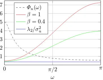
For the example in Section 2.2 for filtered input with n1= 2 ,n2= 3 andna = 1, (41) simplifies to
AsVar ˆG2= λ2 σ2 +
λ2 Φu(ω0)
+ λ2|1 Φu(ω0)
. (42)
0 π/2 π 1
2 3 4 5 6 7
ω Φu(ω)
β= 1 β= 0.4 λ2/σ2
u
Fig. 6. Asymptotic variance of ˆG3(ejω,θˆ2) for β = 1
and β = 0.4. Also shown is λ2/σ 2
, the first term of AsVar ˆG3(ejω,θˆ2) in (42).
6 Optimal correlation structure
In this section we characterize the optimal correlation structure, in order to minimize the total variance. In the previous section, we have seen that not estimating a basis functionkleads to a reduction in variance of the other parameters related to basis functionk. In this section, we will find the optimal correlation structure when the parameterization of the system is such that n1+ 1 = n2 =. . .=nm, i.e., the first module has one parameter
less than the others. Let ˜θ:= [θ2,n2, θ3,n2, . . . , θm,n2]
T,
i.e., the sub vector of parameters related to basis function Bn2(q). Assume the SIMO structure given by (2) and let
the input be white noise with unit variance. Recalling Theorem 7, the covariance matrix of ˆθis given byΛ2:m|1.
In particular, the variance of the entries of ˜θis
AsVar ˆθk,n2 = λk|1
σ2 , k= 2, . . . , m. (43) As before, λk|1is the non-estimable part of ek(t) given
e1(t).
Recalling Theorem 7, the covariance matrix of ˜θis given by σ12Λ2:m|2. The total variance ofθˆ˜is defined as
tvar ˜θ:=
m X
i=2
AsVar ˆθi,n2 = Tr 1
σ2Λ2:m|1.
We are interested in understanding how the correlation ofe1(t) withe2(t), . . . , em(t), i.e.,Λ12 . . . , Λ1m, should
be in order to obtain the minimum value of the above total variance. This problem can be expressed as follows:
minimize
Λ12..., Λ1m
TrΛ2:m|1
s.t. Λ≥0, (44)
where the constraint onΛimplies that not all choices of the entries Λ1i are allowed. Directly characterizing the
noise structure using this formulation of the problem appears to be hard. Therefore, it turns out convenient to introduce an upper triangular Cholesky factorization of Λ, namely define B upper triangular such thatΛ = BBT. Note that
(1) the rows of B, bT
i, i = 1, . . . , m, are such that
kbik2=λi;
(2) E{e1ei}=Λ1i=bT1bi;
(3) there always exists an orthonormal matrixQsuch thatB=ΛCHQ, whereΛCH is the previously
de-fined lower triangular Cholesky factor.
Lemma 20 Let
B=
"
η pT
0 M
#
, M ∈Rm−1×m−1, p∈Rm−1×1, n∈R;
then
Λ2:m|1=M(I− 1 λ1
)ppTMT. (45)
PROOF. See Appendix D.
Using the previous lemma we reformulate (44); keeping M fixed and lettingpvary, we have
maximize
b1
Tr 1 λ1
M ppTMT
s.t. kb1k2=λ1, (46) with bT
1 = [η pT]. Note that the constraint Λ ≥ 0 is automatically satisfied. Let us define v1, . . . , vm−1 as the right-singular vectors ofM, namely the columns of the matrixV in the singular value decomposition (SVD) M =U SVT. The following result provides the structure
ofBthat solves (44).
Theorem 21 Let the input be white noise. Letn1+ 1 = n2=. . .=nm. Then (44)is solved by an upper
triangu-lar Cholesky factorB such that its first row is
b∗T
1 =λ1[0 vT1]. (47)
PROOF. Observe the following facts:
(1) Tr 1
λ1M pp
TMT = 1
λ1p
TMTM p= 1
λ1kM pk 2;
(2) sincebT
1 = [η pT], it is clear that a candidate so-lution to (46) is of the formb∗T
1 = [0 p∗T]. It follows that Problem (46) can be written as
maximize
b1 k
M pk2
whose solution is known to be (a rescaling of) the first right singular vector of M, namely v1. Hence b∗T
1 =
λ1[0 vT
1].
Remark 22 As has been pointed out in Section 2, Λ
is required to be positive definite. Thus, the ideal solu-tion provided by Theorem 21 is not applicable in practice, where one should expect thatη, the first entry ofb1, is
al-ways nonzero. In this case, the result of Theorem 21 can be easily adapted, leading tob∗T
1 =
h
η q1−ηλ21v
T
1
i .
7 Numerical examples
In this section, we illustrate the results derived in the previous sections through three sets of numerical Monte Carlo simulations.
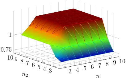
7.1 Effect of model order
Corollary 11 is illustrated in Figure 7, where the follow-ing systems are identified usfollow-ingN = 500 input-output measurements:
Gi= ˜Γiθi, i= 1,2,3 Γ˜i(q) =F(q)−1Γi(q),
Γi(q) = h
B1(q), . . . ,Bni(q)
i
, Bk(q) =q−k, (49)
with
F(q) = 1
1−0.8q−1, θ 0 1=
h
1 0.5 0.7
iT
, θ0
2=
h
1 −1 2
iT
, θ0
3=
h
1 1 2 1 1
iT
.
The input u(t) is drawn from a Gaussian distribution with varianceσ2= 1, filtered byF(q). The measurement noise is normally distributed with covariance matrixΛ= ΛCHΛTCH, where
ΛCH =
1 0 0
0.6 0.8 0 0.7 0.7 0.1
,
thus λ1 = λ2 = λ3 = 1. The sample variance is com-puted using
Cov ˆθs= 1 M C
M C X
k=1
|G3(ejω0, θ0
3)−G3(ejω0,θˆ3)|2,
where M C = 2000 is the number of realizations of the input and noise. The same realizations of the input and noise are used for all model orders.
The variance ofG3(ejω,θˆ3) increases with increasingn i,
i = 1,2, but only up to the point where ni = n3 = 5.
3 4 5 6 7 8 9 10 3
4 5 6 7 8 9 10 0.75
1
n1 n2
Fig. 7. Sample variance ofG3(ejω,θˆ3) as a function of the
number of estimated parameters ofG1andG2.
After that, any increase inn1orn2does not increase the variance ofG3(ejω,θˆ3), as can be seen in Figure 7. The
behavior can be explained by Corollary 11: whenn3 ≥ n1, n2,G3 is the last block, having the highest number of parameters, and any increase in n1, n2 increases the variance ofG3. When for examplen1 ≥n3, the blocks should be reordered so thatG3comes beforeG1. In this case, whenn1 increases the first condition of Corollary 11 does not hold and hence the variance ofG3(ejω,θˆ3)
does not increase further.
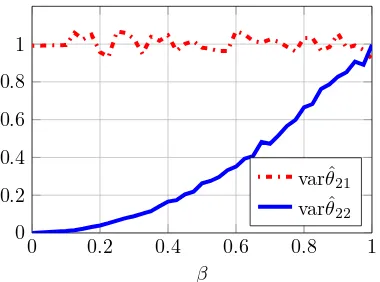
7.2 Effect of removing one parameter
In the second set of numerical experiments, we simulate the same type of system as in Section 2.2. We let β vary in the interval [0.001,1]. For eachβ, we generate M C= 2000 Monte Carlo experiments, where in each of them we collectN = 500 input-output samples. At the i-th Monte Carlo run, we generate new trajectories for the input and the noise and we compute ˆθias in (9). The
sample covariance matrix, for eachβ, is computed as
Cov ˆθs= 1 M C
M C X
i=1
(ˆθi−θ)(ˆθi−θ)T.
Figure 8 shows that the variance of ˆθ21 is always close to one, no matter what the value ofβ is. It also shows that the variance of the estimate ˆθ22 behaves as β2. In particular, whenβ approaches 0 (i.e., almost perfectly correlated noise processes), the variance of such estimate tends to 0. All of the observations are as predicted by Corollary 7 and the example in Section 2.2.
7.3 Optimal correlation structure
A third simulation experiment is performed in order to illustrate Theorem 21. We consider a system withm= 3 outputs; the modules are
0 0.2 0.4 0.6 0.8 1 0
0.2 0.4 0.6 0.8 1
β
varˆθ21 varˆθ22
Fig. 8. Sample variance of the parameters of the first module (as functions ofβ) when the second module has one param-eter.
so that
θ= [θ11θ21θ31θ22θ32]T = [0.3 0.8 0.1 −0.4 0.2]T.
The noise process is generated by the following upper triangular Cholesky factor:
R=
ε √1−ε2cosα √1−ε2sinα
0 0.8 0.6
0 0 1
=
"
ε pT
0 M
#
,
where ε= 0.1 and α∈[0, π] is a parameter tuning the correlation of e1(t) with e2(t) and e3(t). The purpose of this experiment is to show that, whenαis such that p= [√1−ε2cosα √1−ε2sinα]T is aligned with the
first right-singular vectorv1ofM, then the total variance of the estimate of the sub-vector ˜θ= [θ12θ22]T is mini-mized. In the case under analysis,v1= [0.447 0.894]T = [cosα0 sinα0]T, withα0 = 1.11. We letα take values in [0, π] and for eachαwe generateM C= 2000 Monte Carlo runs of N = 500 input-output samples each. We compute the sample total variance of ˜θas
tvar θˆ˜s = M C1
M C X
i=1
(ˆθ22,i−θ22)2+ (ˆθ32,i−θ32)2
,
where ˆθ22,i and ˆθ32,i are the estimates obtained at the
i-th Monte Carlo run.
The results of the experiment are reported in Figure 9. It can be seen that the minimum total variance of the estimate of ˆθis attained for values close toα0 (approx-imations are due to low resolution of the grid of values ofα). An interesting observation regards the value ofα for which the total variance is maximized: this happens when α = 2.68, which yields the second right-singular vector ofM, namelyv2= [−0.894 0.447]T.
0 0.5 1 1.5 2 2.5 3
0 0.4 0.8 1.2 1.6
α var ˆθ2,2+ var ˆθ3,2
Fig. 9. Total sample variance of the parameter vector ˜θ as function ofα.
8 Conclusions
The purpose of this paper has been to examine how the estimation accuracy of a linear SIMO model depends on the correlation structure of the noise and model struc-ture and model order. A formula for the asymptotic covariance of the frequency response function estimate and the model parameters has been developed for the case of temporally white, but possibly spatially corre-lated additive noise. It has been shown that the vari-ance decreases when parts of the noise can be linearly estimated from measurements of other blocks with less estimated parameters. The expressions reveal how the order of the different blocks and the correlation of the noise affect the variance of one block. In particular, it has been shown that the variance of the block of interest levels off when the number of estimated parameters in another block reaches the number of estimated param-eters of the block of interest. The optimal correlation structure for the noise was determined for the case when one block has one parameter less than the other blocks.
References
Ali, M., A. Ali, S.S. Chughtai and H. Werner (2011). Consistent identification of spatially interconnected systems. In ‘Proceedings of the 2011 American Con-trol Conference’. pp. 3583–3588.
Bartlett, M. (1951). ‘An inverse matrix adjustment aris-ing in discriminant analysis’. The Annals of Mathe-matical Statistics22(1), pp. 107–111.
Benesty, J., S. Makino and J. Chen (2005). Speech en-hancement. Springer.
Bertaux, N., P. Larzabal, C. Adnet and E. Chaumette (1999). A parameterized maximum likelihood method for multipaths channels estimation. In ‘Proceedings of the 2nd IEEE Workshop on Signal Processing Ad-vances in Wireless Communications’. pp. 391–394. Chiuso, A. and G. Pillonetto (2012). ‘A Bayesian
Dankers, A., P.M.J. Van den Hof and P.S.C. Heuberger (2013a). Predictor input selection for direct identifica-tion in dynamic networks. In ‘Proceeding of the 52nd IEEE Conference on Decision and Control’. pp. 4541– 4546.
Dankers, A., P.M.J. Van den Hof, X. Bombois and P.S.C. Heuberger (2013b). Predictor input selection for two stage identification in dynamic networks. In ‘Pro-ceeding of the 2013 European Control Conference’. pp. 1422–1427.
Dankers, A., P.M.J. Van den Hof, X. Bombois and P.S.C. Heuberger (2014). Errors-in-variables identification in dynamic networks. In ‘Proceedings of the 19th IFAC World Congress’.
Doclo, S. and M. Moonen (2002). ‘GSVD-based opti-mal filtering for single and multimicrophone speech enhancement’.IEEE Transactions on Signal Process-ing50(9), 2230–2244.
Everitt, N., C.R. Rojas and H. Hjalmarsson (2013). A geometric approach to variance analysis of cascaded systems. In ‘Proceedings of the 52nd IEEE Conference on Decision and Control’.
Gevers, M., L. Miˇskovi´c, D. Bonvin and A. Karimi (2006). ‘Identification of multi-input systems: vari-ance analysis and input design issues’. Automatica
42(4), 559 – 572.
Gunes, B., A. Dankers and P.M.J. Van den Hof (2014). A variance reduction technique for identification in dynamic networks. In ‘Proceedings of the 19th IFAC World Congress’.
Haber, A. and M. Verhaegen (2014). ‘Subspace identi-fication of large-scale interconnected systems’. IEEE Transactions on Automatic Control 59(10), 2754– 2759.
H¨agg, P., B. Wahlberg and H. Sandberg (2011). On iden-tification of parallel cascade serial systems. In ‘Pro-ceedings of the 18th IFAC World Congress’.
Hjalmarsson, H. and B. Ninness (2006). ‘Least-squares estimation of a class of frequency functions: A finite sample variance expression’.Automatica42(4), 589 – 600.
Hjalmarsson, H. and J. M˚artensson (2011). ‘A geomet-ric approach to variance analysis in system identi-fication’. IEEE Transactions on Automatic Control
56(5), 983 –997.
Horn, R. and C.R. Johnson (1990). Matrix Analysis. Cambridge University Press.
Koski, T. and J. Noble (2012). ‘A review of Bayesian networks and structure learning’.Mathematica Appli-canda40(1), 51–103.
Ljung, L. (1985). ‘Asymptotic variance expressions for identified black-box transfer function models’. IEEE Transactions on Automatic Control30(9), 834 – 844. Ljung, L. (1999). System Identification: Theory for the
User. 2 edn. Prentice Hall.
Ljung, L. and P.E. Caines (1980). ‘Asymptotic normality of prediction error estimators for approximate system models’.Stochastics3(1-4), 29–46.
Ljung, L., H. Hjalmarsson and H. Ohlsson (2011).
‘Four encounters with system identification’. Euro-pean Journal of Control17(5), 449–471.
M˚artensson, J. (2007). Geometric analysis of stochastic model errors in system identification. Ph.D. thesis. KTH, Automatic Control.
Materassi, D., M.V. Salapaka and L. Giarre (2011). Rela-tions between structure and estimators in networks of dynamical systems. In ‘Proceedings of the 50th IEEE Conference on Decision and Control and European Control Conference’. pp. 162–167.
McCombie, D., A.T. Reisner and H.H. Asada (2005). ‘Laguerre-model blind system identification: Cardio-vascular dynamics estimated from multiple peripheral circulatory signals’. IEEE Transactions on Biomedi-cal Engineering52(11), 1889–1901.
Ninness, B. and F. Gustafsson (1997). ‘A unifying con-struction of orthonormal bases for system identifi-cation’. IEEE Transactions on Automatic Control
42, 515–521.
Ninness, B. and H. Hjalmarsson (2004). ‘Variance er-ror quantifications that are exact for finite model order’. IEEE Transactions on Automatic Control
49(8), 1275–1291.
Ninness, B. and H. Hjalmarsson (2005a). ‘Analysis of the variability of joint input–output estimation methods’.
Automatica41(7), 1123 – 1132.
Ninness, B. and H. Hjalmarsson (2005b). ‘On the fre-quency domain accuracy of closed-loop estimates’.
Automatica41, 1109–1122.
Ninness, B., H. Hjalmarsson and F. Gustafsson (1999). ‘The fundamental role of general orthonormal bases in system identification’.IEEE Transactions on Au-tomatic Control44(7), 1384–1406.
Ramazi, P., H. Hjalmarsson and J. M˚artensson (2014). ‘Variance analysis of identified linear MISO mod-els having spatially correlated inputs, with applica-tion to parallel Hammerstein models’. Automatica
50(6), 1675 – 1683.
Schmidt, R. (1986). ‘Multiple emitter location and sig-nal parameter estimation’.IEEE Transactions on An-tennas and Propagation34(3), 276–280.
S¨oderstr¨om, T. and P. Stoica (1989).System identifica-tion. Prentice-Hall. Englewood Cliffs.
Stoica, P., M. Viberg and B. Ottersten (1994). ‘Instru-mental variable approach to array processing in spa-tially correlated noise fields’. IEEE Transactions on Signal Processing42(1), 121–133.
Torres, P., J.W. van Wingerden and M. Verhaegen (2014). ‘Output-error identification of large scale 1d-spatially varying interconnected systems’. IEEE Transactions on Automatic Control60(1), 130–142. Trefethen, L. and D. Bau (1997).Numerical Linear
Alge-bra. Society for Industrial and Applied Mathematics. Trudnowski, D., J.M. Johnson and J.F. Hauer (1998). SIMO system identification from measured ring-downs. In ‘Proceedings of the 1998 American Control Conference’. Vol. 5. pp. 2968–2972.
records’. Earthquake Engineering & Structural Dy-namics40(6), 661–674.
Van den Hof, P. M. J., Arne Dankers, P. S. C. Heuberger and X Bombois (2013). ‘Identification of dynamic models in complex networks with prediction error methods - basic methods for consistent module esti-mates’.Automatica49(10), 2994–3006.
Viberg, M. and B. Ottersten (1991). ‘Sensor array pro-cessing based on subspace fitting’.IEEE Transactions on Signal Processing39(5), 1110–1121.
Viberg, M., P. Stoica and B. Ottersten (1997). ‘Max-imum likelihood array processing in spatially corre-lated noise fields using parameterized signals’. IEEE Transactions on Signal Processing45(4), 996–1004. Wahlberg, B., H. Hjalmarsson and J. M˚artensson (2009).
‘Variance results for identification of cascade systems’.
Automatica45(6), 1443–1448.
Yuan, Z. D. and L. Ljung (1984). ‘Black-box identifi-cation of multivariable transfer functions–asymptotic properties and optimal input design’. International Journal of Control40(2), 233–256.
Zhu, Y. (1989). ‘Black-box identification of MIMO trans-fer functions: Asymptotic properties of prediction er-ror models’.International Journal of Adaptive Control and Signal Processing3(4), 357–373.
Zhu, Y. (2001). Multivariable system identification for process control. Elsevier.
A Proof of Lemma 5
Let v(t) = Λ−1CHe(t) for some real valued random vari-able e(t) (Λ−1CH exists and is unique for Λ > 0 (Horn and Johnson, 1990)). Then Cov v(t) = I. Similarly e(t) = ΛCHv(t). The set {v1(t), . . . , vj(t)} is a
func-tion of e1(t), . . . , ej(t) only and vice versa, for all
1 ≤ j ≤ m. Thus, if e1(t), . . . , ej(t) are known, then
also{v1(t), . . . , vj(t)} are known, but nothing is known
about {vj+1(t), . . . , vm(t)}. Thus, for j < i the best
linear estimator ofei(t) givene1(t), . . . , ej(t), is
ˆ ei|j(t) =
j X
k=1
γikvk(t), (A.1)
and
ei(t)−eˆi|j(t)
has variance
λi|j= i X
k=j+1 γ2ik.
For the last part of the lemma, we realize that the de-pendence of ˆei|j(t) onej(t) in Equation (A.1) is given by
γij/γjj(sincev1(t), . . . , vj−1(t) do not depend onej(t)).
Hence ˆei|j(t) depends onej(t) if and only ifγij 6= 0.
B Proof of Theorem 10
Before giving the proof of Theorem 10 we need the fol-lowing auxiliary lemma.
Lemma 23 Let Λ >0and real and its Cholesky factor
ΛCH be partitioned according toe1:χk−1andeχk:m,
Λ=
"
Λ1 Λ12 Λ21 Λ2
#
, ΛCH =
"
(ΛCH)1 0
(ΛCH)21 (ΛCH)2 #
.
Then
Λχk:m|χk−1= (ΛCH)2(ΛCH)
T
2.
PROOF. By the derivations of Lemma A, for some v(t) with Covv(t) = I, e(t) = ΛCHv(t) and v1:χ−1(t)
are known since e1:χ−1(t) are known. Furthermore
ˆ
eχk:m|χk−1(t) = (ΛCH)21v1:χ−1(t), which implies eχk:m|χk−1(t)−eˆχk:m|χk−1(t) = (ΛCH)2vχk:m(t) and the results follows since Covvχk:m(t) =I.
The asymptotic variance is given by (11) with
Ψ(q) = ˜Ψ(q)Λ−T CH.
Letn=n1+· · ·+nm. From the upper triangular
struc-ture ofΛ−CHT andn1 ≤n2 ≤. . .≤nm, an orthonormal
basis forSΨ, the subspace spanned by the rows ofΨ, is
given by
BSk(ejω) := h
Bk 0 . . . 0 i
, k=1, . . . , n1 BSk(ejω) :=
h
0 Bk−n1 0 . . .
i
, k=n1+ 1, . . . , n2 ..
. (B.1)
BSk(ejω) := h
. . . 0 Bk−n+nm
i
, k=n−nm+1, . . . , n.
First note that
∂G ∂θ =Ψ Λ
T CH.
Then, using Theorem 3,
σ2AsVar ˆG=ΛCH n X
k=1
BSk(ejω0)
∗
BSk(ejω0)ΛTCH.
Sorting the sum with respect to the basis functions Bk(ejω0), we get
σ2AsCov ˆGi =ΛCH nm
X
k=1
|Bk(ejω0)|2 "
0χk−1 0
0 I
#
Using Lemma 23
AsCov ˆG= 1 σ2
nm
X
k=1
"
0χk−1 0
0 Λχk:m|χk−1
#
|Bk(ejω0)|2.
Thus (25) follows. We now show the first part of the theorem, that
AsCov ˆθ¯= 1
σ2diag(Λ1:m, Λχ2:m|χ2−1, . . . , Λχnm:m|χnm−1). The covariance of ˆGcan be expressed as
AsCov ˆG=TAsCov ˆθ T¯ ∗ (B.2) where
T =hB1I(1) B2I(2). . . BnmI(nm)
i
,
I(k) =
"
0 Im−χk+1
#
∈Rm×(m−χk+1).
However, (B.2) equals (25) for all ω and the theorem follows.
C Proof of Corollary 11
To prove Corollary 11 we will use (28). First, we make the assumption that j is the last module that has nj
parameters. This assumption is made for convenience since reordering all modules withnjestimated
parame-ters does not change (28). First of all, we see that if
nj ≥ni,
then (28) does not increase whennjincreases. If instead
nj < ni,
the increase in variance is given by
γij2|Bnj+1(e
jω0) |2,
which is non-zero iff γij 6= 0 and |Bnj+1(e
jω0)|2 6= 0. From Lemma 5 the theorem follows.
D Proof of Lemma 20
The inverse ofB is
B−1=
"
η−1 −qT
0 M−1
#
, qT :=η−1pTM−1,
so that
Λ−1=B−TB−1=
"
η−2 −qTη−1 −qη−1 M−TM−1+qqT
#
.
Hence, using the Sherman–Morrison formula (Bartlett, 1951)
Λ2:m|1= M−TM−1+qqT
−1
=M MT −1kM MTqqTM MT =M MT −1kM pp
TMT
η2 ,
where
k= 1 +qTM MTq= 1 + p
Tp
η2 = η
2+pTp
η2 =
kb1k22 η2 = λ1