Empirical Comparison of ML and UMVU Estimators of the Generalized Variance for some Normal Stable Tweedie Models: a Simulation Study

(1)

https://doi.org/10.12988/ams.2016.69238

Empirical Comparison of ML and UMVU Estimators

of the Generalized Variance for some Normal

Stable Tweedie Models: a Simulation Study

Khoirin Nisa1

Department of Mathematics, Lampung University, Indonesia

C´elestin C. Kokonendji

Laboratoire de Mathématiques de Besan¸con Université Bourgogne Franche-Comté, France

Asep Saefuddin, Aji Hamim Wigena

Department of Statistics, Bogor Agricultural University, Indonesia

I Wayan Mangku

Department of Mathematics, Bogor Agricultural University, Indonesia

Copyright c2016 Khoirin Nisa, C´elestin C. Kokonendji, Asep Saefuddin, Aji Hamim Wigena and I Wayan Mangku. This article is distributed under the Creative Commons Attribution License, which permits unrestricted use, distribution, and reproduction in any medium, provided the original work is properly cited.

Abstract

This paper discuss a comparison of the maximum likelihood (ML) estimator and the uniformly minimum variance unbiased (UMVU) es-timator of generalized variance for some normal stable Tweedie models through simulation study. We describe the estimation of some particular cases of multivariate NST models, i.e. normal gamma, normal Poisson

1_{Also affiliated to Bogor Agricultural University, Indonesia and Universit´e Bourgogne}

(2)

and normal invers-Gaussian. The result shows that UMVU method pro-duces better estimations than ML method on small samples and they both produce similar estimations on large samples.

Mathematics Subject Classification: 62H12

Keywords: Multivariate natural exponential family, variance function, maximum likelihood, uniformly minimum variance unbiased

1 Introduction

Normal stable Tweedie (NST) models were introduced by Boubacar Ma¨ınassara and Kokonendji [3] as the extension of normal gamma [5] and normal inverse Gaussian [4] models. NST models are composed by a fixed univariate stable Tweedie variable having a positive value domain, and the remaining random variables given the fixed one are real independent Gaussian variables with the same variance equal to the fixed component. For a k-dimensional (k _≥ 2) NST random vectorX= (X1, . . . , Xk)⊤, the generatingσ-finite positive

mea-sure να,t is given by

να,t(dx) = ξα,t(dx1)

k

Y

j=2

ξ2,x1(dxj), (1)

whereξα,tis the well-known probability measure of univariate positiveσ-stable

distribution generating L´evy process (Xα

t)t>0 which was introduced by Feller [7] as follows

ξα,t(dx) =

1 πx

∞ X

r=0

tr_{Γ(1 +}_αr)sin(₋_rπα)

r!αr_(α₋₁₎−_r_[(1

−α)x]αr1x>0dx=ξα,t(x)dx. (2)

Here α _∈ (0,1) is the index parameter, Γ(.) is the classical gamma function, and I_A _{denotes the indicator function of any given event A that takes the}

value 1 if the event accurs and 0 otherwise. Paremeterα can be extended into α _∈ (_−∞,2] [10]. For α = 2 in (2), we obtain the normal distribution with density

ξ2,t(dx) =

1

√

2πtexp

−x2 2t

dx.

(3)

1. Normal gamma(NG). Forα = 0 in (1) one has the generating measure of normal gamma as follows:

ν0,t(dx) =

It is a member of simple quadratic natural exponential families (NEFs) [6] and was called as ”gamma-Gaussian” which was characterized by Kokonendji and Masmoedi [8].

2. Normal invers Gaussian (NIG). Forα = 1/2 in (1) we can write the normal inverse Gaussian generating measure as follows

ν1/2,t(dx) = It was introduced as a variance-mean mixture of a univariate inverse Gaussian with multivariate Gaussian distribution [4] and has been used in finance (see e.g. [1, 2]).

3. Normal Poisson (NP). For the limit case α=_−∞in (1) we have the so-called normal Poisson generating measure

ν−∞,t(dx) = Since it is also possible to have x1 = 0 in the Poisson part, the correspond-ing normal Poisson distribution is degenerated as δ0. This model is recently characterized by Nisa et al. [9]

2 Generalized Variance of NST Models

The cumulant function Kνα,t(θ) = log

Rkexp(θx)ξα,t(dx) is the cumulant function of the

(4)

discuss here the corresponding cumulant function is given by

(see [3, Section 2]). The cumulant function is finite forθ in canonical domain

Θ(να,t) ={θ ∈Rk;θ1+ 1₂

ance function which is the variance-covariance matrix in term of mean param-eterization;P(µ;Gα,t) :=P[θ(µ);να,t]; is obtained through the second

deriva-tive of the cumulant function, i.e. VG_α,t(µ) = K′′_ν

α,t[θ(µ)] whereµ=K

′

να,t(θ).

Then calculating the determinant of the variance function will give the gen-eralized variance. We summarize the variance function and the gengen-eralized variance of NG, NIG and NP models in Table 1.

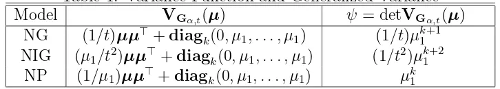
Table 1: Variance Function and Generalized Variance

Model VG_α,t(µ) ψ = detVG_α,t(µ)

NG (1/t)µµ⊤

+diag_k(0, µ1, . . . , µ1) (1/t)µk1+1 NIG (µ1/t2)µµ⊤+diagk(0, µ1, . . . , µ1) (1/t2)µk1+2

NP (1/µ1)µµ⊤+diagk(0, µ1, . . . , µ1) µk1

The ML and UMVU estimators of the generalized variance in Table 1 are stated in the following proposition.

Proposition 1 LetX1, . . . , Xnbe random vectors with distributionP(θ;α, t)∈

G(νp,t)in a given NST family. DenotingX = (X1+. . .+Xn)/n= (X1, . . . , Xk)T

the sample mean with positive first component X1, the ML estimator of the generalized variance of NG, NP and NIG models is given by:

(5)

and the UMVU estimator is given by (see Boubacar Ma¨ınassara and Kokonendji , [3])

3 Simulation Study

In order to examine the behavior of ML and UMVU estimators empirically we carried out a simulation study. We run Monte-Carlo simulations using R software. We set several sample sizes (n) varied from 3 to 1000 and we generated 1000 samples for eachn. We considerk = 2,4,6 to see the effects of kon generalized variance estimations. For simplicity we setµ1 = 1. Moreover, to see the effect of zero values proportion within X1 in the case of normal Poisson, we also consider small mean values on the Poisson component i.e. µ1 = 0.5 because P(X1 = 0) = exp(−µ1).

We report the numerical results of the generalized variance estimations for each model, i.e. the empirical expected value of the estimators with its standard errors (Se) and the empirical mean square error (MSE). We calculated the mean square error (MSE) of each method over 1000 data sets using the following formula:

We generated normal gamma distribution samples using the generatingσ-finite positive measureνα,tof normal gamma in (1). Table 2 show the expected values

of generalized variance estimates with their standard errors (in parentheses) and the means square error values of both ML and UMVU methods in case of normal gamma.

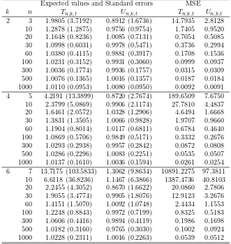
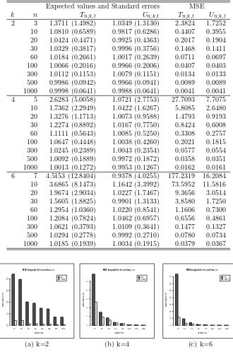
From the result in Table 2 we can observe different performances of ML estimator (Tn;k,t) and UMVU estimator (Un;k,p,t) of the generalized variance.

The expected values of Tn;k,t converge while the values of Un;k,t do not, but

(6)

for n _≤ 30, this shows that UMVU is an unbiased estimator while ML is an asymtotically unbiased estimator. For the two methods, the standar error of the estimates decreases when the sample size increase.

Table 2: The expected values (with empirical standard errors) and MSE of Tn;k,tandUn;k,tfor normal-gamma with 1000 replications for given target value

µk₁+1 = 1 with k _{∈ {}2,4,6_}.

Expected values and Standard errors MSE

k n T_n_;_k,t U_n_;_k,t T_n_;_k,t U_n_;_k,t

2 3 1.9805 (3.7192) 0.8912 (1.6736) 14.7935 2.8128 10 1.2878 (1.2875) 0.9756 (0.9754) 1.7405 0.9520 20 1.1648 (0.8236) 1.0085 (0.7131) 0.7054 0.5085 30 1.0998 (0.6031) 0.9978 (0.5471) 0.3736 0.2994 60 1.0380 (0.4115) 0.9881 (0.3917) 0.1708 0.1536 100 1.0231 (0.3152) 0.9931 (0.3060) 0.0999 0.0937 300 1.0036 (0.1774) 0.9936 (0.1757) 0.0315 0.0309 500 1.0076 (0.1365) 1.0016 (0.1357) 0.0187 0.0184 1000 1.0110 (0.0953) 1.0080 (0.0950) 0.0092 0.0091 4 5 4.2191 (13.3899) 0.8720 (2.7674) 189.6509 7.6750 10 2.3799 (5.0869) 0.9906 (2.1174) 27.7810 4.4837 20 1.6461 (2.0572) 1.0328 (1.2906) 4.6494 1.6668 30 1.3831 (1.3505) 1.0066 (0.9828) 1.9707 0.9660 60 1.1904 (0.8014) 1.0117 (0.6811) 0.6784 0.4640 100 1.0869 (0.5706) 0.9849 (0.5171) 0.3332 0.2676 300 1.0293 (0.2938) 0.9957 (0.2842) 0.0872 0.0808 500 1.0286 (0.2296) 1.0083 (0.2251) 0.0535 0.0507 1000 1.0137 (0.1610) 1.0036 (0.1594) 0.0261 0.0254 6 7 13.7175 (103.5833) 1.3062 (9.8634) 10891.2275 97.3811

10 6.6118 (36.8236) 1.1467 (6.3866) 1387.4736 40.8103 20 2.2455 (4.3052) 0.8670 (1.6622) 20.0860 2.7806 30 1.9055 (3.4774) 0.9905 (1.8076) 12.9123 3.2676 60 1.4151 (1.5070) 1.0092 (1.0748) 2.4434 1.1553 100 1.2248 (0.8843) 0.9972 (0.7199) 0.8325 0.5183 300 1.0606 (0.4416) 0.9894 (0.4119) 0.1986 0.1698 500 1.0182 (0.3160) 0.9765 (0.3030) 0.1002 0.0924 1000 1.0228 (0.2311) 1.0016 (0.2263) 0.0539 0.0512

(7)

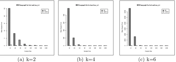
10 20 30 60 100 300 500 1000 ML UMVU

MSE bargraph for k=2 and mu_j=1

Sample Size

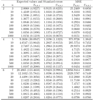
The result for normal inverse-Gaussian is presented in Table 3. Similar with normal gamma, the result for normal inverse-Gaussian shows that UMVU method produced better estimates than ML method for small sample sizes. From the result we can conclude that the two estimators are consistent. The bargraph of MSE values forn_≥10 in Table 3 is presented in Figure 2. Notice that the result for this case is similar to the normal gamma case, i.e. for small sample sizes the difference between the MSEs of ML and UMVU estimators for normal inverse-Gaussian also increases when k increases.

10 20 30 60 100 300 500 1000 ML UMVU

Sample Size

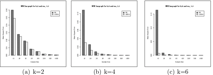
The simulation results for normal Poisson are presented in Table 4 and Table 5 for µ1 = 1 and µ1 = 0.5 respectively. In this simulation, the proportion of zero values in the samples increases when the mean of the Poisson component becomes smaller. For normal-Poisson distribution with µj = 0.5, we have

(8)

Table 3: The expected values (with standar errors) and MSE of Tn;k,t and

Un;k,t for normal inverse-Gaussian with 1000 replications for given target value

µk₁+2 = 1 andk _{∈ {}2,4,6_}.

2 3 2.0068 (4.9227) 0.9135 (0.8235) 25.2469 0.6856 10 1.4249 (2.8513) 1.0316 (0.4388) 8.3103 0.1935 20 1.5936 (1.8951) 1.1340 (0.3718) 3.9439 0.1562 30 1.3677 (1.0155) 1.1641 (0.2668) 1.1664 0.0981 60 1.0846 (0.5341) 1.1104 (0.1856) 0.2924 0.0466 100 1.0819 (0.5166) 1.1102 (0.1675) 0.2735 0.0402 300 1.0006 (0.2570) 1.0843 (0.0919) 0.0660 0.0156 500 1.0356 (0.1890) 1.1374 (0.0727) 0.0370 0.0242 1000 1.0156 (0.1219) 1.0116 (0.0670) 0.0151 0.0115 4 5 9.3836 (30.0947) 1.3196 (1.1323) 975.9726 1.3843 10 4.6547 (13.8643) 1.2837 (0.8153) 205.5754 0.7452 20 2.7487 (5.1845) 1.2963 (0.6189) 29.9373 0.4709 30 1.4822 (2.1166) 1.1854 (0.4572) 4.7125 0.2434 60 1.3095 (1.1051) 1.2560 (0.3054) 1.3170 0.1588 100 1.1673 (0.8467) 1.2264 (0.2671) 0.7449 0.1226 300 1.0849 (0.4296) 1.2542 (0.1520) 0.1918 0.0877 500 1.0350 (0.2839) 1.0762 (0.0914) 0.0818 0.0416 1000 1.0107 (0.2080) 1.0102 (0.1137) 0.0434 0.0337 6 7 20.4865 (113.4633) 0.9423 (0.9984) 12056.9414 1.0001 10 12.1032 (55.7841) 1.0596 (0.8610) 2329.5787 0.7449 20 3.4498 (10.3056) 1.0054 (0.5933) 112.2060 0.3520 30 2.1422 (3.2262) 1.0246 (0.4970) 11.7130 0.2476 60 1.8236 (2.6064) 1.0587 (0.3744) 7.4717 0.1436 100 1.2468 (1.1599) 1.0129 (0.2643) 1.4062 0.1170 300 1.0781 (0.4953) 1.0568 (0.1596) 0.2514 0.0929 500 1.0815 (0.4065) 1.0230 (0.1110) 0.1719 0.0922 1000 1.0207 (0.2816) 1.0204 (0.0775) 0.0798 0.0760

generalized variance estimation as we can see that Tn;k,t and Un;k,t have the

same behavior for both values of µ1.

The MSE in Table 4 and 5 forn _≥10 are displayed as bargraphs presented in Figure 3 and Figure 4. From those figures we see that UMVU is preferable than ML because it always has smaller MSE values when sample sizes are small (n 630).

4 Conclusion

(9)

Table 4: The expected values (with standar errors) and MSE ofTn;k,tandUn;k,t

for normal Poisson with 1000 replications for given target value µk

1 = 1 and k_{∈ {}2,4,6_}.

2 3 1.3711 (1.4982) 1.0349 (1.3130) 2.3824 1.7252 10 1.0810 (0.6589) 0.9817 (0.6286) 0.4407 0.3955 20 1.0424 (0.4471) 0.9925 (0.4363) 0.2017 0.1904 30 1.0329 (0.3817) 0.9996 (0.3756) 0.1468 0.1411 60 1.0184 (0.2661) 1.0017 (0.2639) 0.0711 0.0697 100 1.0066 (0.2016) 0.9966 (0.2006) 0.0407 0.0403 300 1.0112 (0.1153) 1.0079 (0.1151) 0.0134 0.0133 500 0.9986 (0.0942) 0.9966 (0.0941) 0.0089 0.0089 1000 0.9998 (0.0641) 0.9988 (0.0641) 0.0041 0.0041 4 5 2.6283 (5.0058) 1.0721 (2.7753) 27.7093 7.7075 10 1.7362 (2.2949) 1.0422 (1.6267) 5.8085 2.6480 20 1.3276 (1.1713) 1.0073 (0.9588) 1.4793 0.9193 30 1.2274 (0.8892) 1.0167 (0.7750) 0.8424 0.6008 60 1.1111 (0.5643) 1.0085 (0.5250) 0.3308 0.2757 100 1.0647 (0.4448) 1.0038 (0.4260) 0.2021 0.1815 300 1.0245 (0.2389) 1.0043 (0.2354) 0.0577 0.0554 500 1.0092 (0.1889) 0.9972 (0.1872) 0.0358 0.0351 1000 1.0013 (0.1272) 0.9953 (0.1267) 0.0162 0.0161 6 7 4.5153 (12.8404) 0.9378 (4.0255) 177.2319 16.2084 10 3.6865 (8.1473) 1.1642 (3.3992) 73.5952 11.5816 20 1.9674 (2.9034) 1.0227 (1.7467) 9.3656 3.0514 30 1.5605 (1.8825) 0.9901 (1.3133) 3.8580 1.7250 60 1.2954 (1.0360) 1.0220 (0.8541) 1.1606 0.7300 100 1.2084 (0.7824) 1.0462 (0.6957) 0.6556 0.4861 300 1.0621 (0.3793) 1.0109 (0.3641) 0.1477 0.1327 500 1.0294 (0.2778) 0.9992 (0.2710) 0.0780 0.0734 1000 1.0185 (0.1939) 1.0034 (0.1915) 0.0379 0.0367

10 20 30 60 100 300 500 1000 ML UMVU

MSE bargraph for k=2 and mu_1=1

Sample Size

(10)

Table 5: The expected values (with standard errors) and MSE of Tn;k,t and

Un;k,tfor normal Poisson with 1000 replications for given target valueµk1 = 0.5k and k_{∈ {}2,4,6_}.

2 3 0.3930 (0.5426) 0.2320 (0.4223) 0.3148 0.1787 10 0.2868 (0.2421) 0.2378 (0.2212) 0.0600 0.0491 20 0.2652 (0.1660) 0.2407 (0.1583) 0.0278 0.0251 30 0.2642 (0.1374) 0.2476 (0.1332) 0.0191 0.0177 60 0.2598 (0.0903) 0.2514 (0.0888) 0.0083 0.0079 100 0.2534 (0.0712) 0.2484 (0.0705) 0.0051 0.0050 300 0.2495 (0.0418) 0.2478 (0.0417) 0.0017 0.0017 500 0.2491 (0.0313) 0.2482 (0.0313) 0.0010 0.0010 1000 0.2495 (0.0221) 0.2490 (0.0221) 0.0005 0.0005

4 5 0.2999 (0.8462) 0.0685 (0.3474) 0.7724 0.1207 10 0.1696 (0.3115) 0.0689 (0.1750) 0.1085 0.0306 20 0.1089 (0.1541) 0.0658 (0.1097) 0.0259 0.0120 30 0.0886 (0.0894) 0.0617 (0.0689) 0.0087 0.0048 60 0.0774 (0.0559) 0.0642 (0.0487) 0.0033 0.0024 100 0.0704 (0.0403) 0.0627 (0.0370) 0.0017 0.0014 300 0.0643 (0.0207) 0.0618 (0.0201) 0.0004 0.0004 500 0.0635 (0.0158) 0.0620 (0.0156) 0.0003 0.0002 1000 0.0631 (0.0115) 0.0624 (0.0114) 0.0001 0.0001

6 7 0.2792 (1.2521) 0.0268 (0.2274) 1.6371 0.0519 10 0.1212 (0.3918) 0.0165 (0.0858) 0.1646 0.0074 20 0.0427 (0.0883) 0.0124 (0.0345) 0.0085 0.0012 30 0.0356 (0.0539) 0.0151 (0.0271) 0.0033 0.0007 60 0.0236 (0.0281) 0.0149 (0.0196) 0.0009 0.0004 100 0.0211 (0.0183) 0.0159 (0.0145) 0.0004 0.0002 300 0.0173 (0.0089) 0.0157 (0.0082) 0.0001 0.0001 500 0.0166 (0.0068) 0.0157 (0.0064) 0.0000 0.0000 1000 0.0164 (0.0044) 0.0159 (0.0043) 0.0000 0.0000

for the three models show that UMVU produces better estimation than ML for small sample sizes. However, the two methods are consistent and they become more similar when the sample size increases.

References

(11)

10 20 30 60 100 300 500 1000 ML UMVU

Sample Size

[2] J. Andersson, On the normal inverse Gaussian stochastic volatility model, Journal of Business & Economic Statistics, 19 (2001), no. 1, 44-54. https://doi.org/10.1198/07350010152472607

[3] Y. Boubacar Ma¨ınassara and C. C. Kokonendji, On normal stable Tweedie models and power-generalized variance functions of only one component, TEST, 23 (2014), 585-606. https://doi.org/10.1007/s11749-014-0363-9 [4] O. E. Barndorff-Nielsen, J. Kent and M. Sørensen, Normal variance-mean

mixtures and z distributions,International Statistical Review, 50 (1982), 145-159. https://doi.org/10.2307/1402598

[5] J. M. Bernardo and A. F. M. Smith, Bayesian Theory, Wiley, New York, 1993. https://doi.org/10.1002/9780470316870

[6] M. Casalis, The 2d+ 4 simple quadratic natural exponential families on

Rd_, _{The Annals of Statistics}_,₂₄ _{(1996), 1828-1854.}

https://doi.org/10.1214/aos/1032298298

[7] W. Feller, An Introduction to Probability Theory and its Applications Vol. II, Second edition, Wiley, New York, 1971.

[8] C. C. Kokonendji and A. Masmoudi, On the Monge-Amp`ere equation for characterizing gamma-Gaussian model,Statistics and Probability Letters, 83 (2013), 1692-1698. https://doi.org/10.1016/j.spl.2013.03.023

[9] K. Nisa, C.C. Kokonendji and A. Saefuddin, Characterizations of multi-variate normal Poisson model, Journal of Iranian Statistical Society, 14 (2015), 37-52.

(12)

Eds. J. K. Ghosh and J. Roy, Indian Statistical Institute, Calcutta, 1984, 579–604.