Analysis of Variance for Attribute Data in Taguchi ‘s Approach Zurnila Marli Kesuma, M.Si
Department of mathematics, Syiah Kuala University, Banda aceh, Indonesia kesumaku@yahoo.com
Abstract. Taguchi has extended the audio concept of the signal-to-noise ratio (SN ratio) to experiments involving many factors. The formula for signal-to-noise ratio are designed so that an experimenter can always select the largest factor level setting to optimize the quality characteristic of an experiment. When the quality characteristic is a proportion, such as the fraction defective, denoted p, which can take values between 0 and 1, we use the omega (Ω) transformation as an objective characteristics. The selection of important factor is not only based on the response table, but also uses attribute accumulation analysis - analysis of variance and the contribution ratio to establish significant factors. The method of conducting the analysis of variance is create a table of data, Calculate the overall total sum of squares due to class I and class II. Calculate the total degree of freedom. Draw the analysis of variance. Calculate the predicted optimum process and calculate the confidence interval of a predicted mean.
2000 Mathematics Subject Classification: 30C45, Secondary 30C80
Keywords : omega(Ω) transformation, analysis of variance,contribution ratio.
1. Introduction
Analysis variance (ANOVA) was first introduced by Sir Ronald Fisher. It is a method of partitioning variability into identifiable sources of variation and the associated degrees of freedom in an experiment. Taguchi recommends that statistical experimental design method be employed to assist in quality improvement, particularly during parameter design and tolerance design, specifically to reduce the variability. He proposed some steps in analysis varians, that is calculate the percent contribution and pool insignificant factors.
Attribute data analysis such as the fraction defective, denoted p, can take values between 0 and 1. Frequently, p is expressed as a percentage where it can take values between 0% and 100%. With fraction defective, the best value for p is zero. Attribute accumulation is used when the experimental data can be ranked or categorized.
Attribute accumulation analysis uses analysis of variance and the contribution ratio to establish significant factors.
2. Fraction Defective Analysis and Weighting
determining the totals for each factor level in each category. For each factor, the total of the data in level 1 and level 2 should be the same.
Fraction defective of each class can be formulated as follows :
( )III I III II I I I f f f f f f p = + + =
( )III II III II I II I
f
f
f
f
f
f
p
=
+
+
=
( )III III III II I III III
f
f
f
f
f
f
p
=
+
+
=
(2.1)Accumulation analysis needs some understanding of the binomial distribution. If the fraction defective is p, then the corresponding variance is:
2
σ
= p x (1-p) (2.2)This implies that the variance depends on p. However, if we are to compare two distributions (corresponding to classes or categories in an experiment), we can only make a fair comparison if the varians are approximately the same. Since, the sum of squares of different Classes in accumulation analysis analysis would have different bases, it is important to normalize these basis, by dividing the sum of squares of each class by its variance. This procedur is frequently called weighting. The weight of each class is:
)
1
(
1
1
1 21
P
Ix
P
I
=
σ
=
−
ω
(2.3)For ease of calculation, it may be better to use:
)
1
(
1
1
1 21
P
Ix
P
I
=
σ
=
−
ω
⎟ ⎟ ⎠ ⎞ ⎜ ⎜ ⎝ ⎛ − = ) ( ) ( 1 1 III I III I f f x f f ⎟ ⎟ ⎠ ⎞ ⎜ ⎜ ⎝ ⎛ − = ) ( ) ( ) ( 1 III I III III I f f f x f f)
(
( ) 2 ) ( I III I IIIf
f
x
f
f
−
)
(
( ) 2 ) ( II III II III IIf
f
x
f
f
−
=
ω
(2.5)3. The Analysis of Variance
From the attribute accumulation, The fraction defective analysis needs some quantities to conduct the analysis of Variance. And the following quantity should be calculated.
3.1 The Total Sum of Squares Due To Class I S1= total sum of squares of class I
I
III
f
f
f
⎟
⎟
ω
⎠
⎞
⎜
⎜
⎝
⎛
−
=
) ( 2 1 1(
)
I III III III III If
f
x
f
f
x
f
f
f
f
−
−
=
) ( 1 2 ) ( ) ( 2 1 ) ()
(
)
(
) ( 2 ) ( ) ( ) ( I III I III III I III If
f
x
f
f
x
f
f
f
x
f
−
−
=
=
f
(III) (3.1)Similarly, the total sum of squares of class II is also
f
(III)a. The Overall Total Sum of Squares Due To Class I and Class II ST = total sum of squares of class I and class II
=
f
(III)+
f
(III) (3.2)In general :
ST = total sum of squares of class I and class II
=( total number of measurements) x (number of classes - 1)
3.3 The Degrees of Freedom Due To Class I The degrees of freedom of class I is vI.
1
)
(
−
=
IIII
f
v
(3.3)Similarly, the degrees of freedom of class II is also
f
(III)−
1
3.4 The Total Degrees of Freedom
=
vT total degrees of freedom of class I dan class II (3.4) =
(
f
(III)−
1
)
+
(
f
(III)−
1
)
In general:
=
vT total degrees of freedom of class I dan class II
= (total number of measurements -1) x (number of classes -1) 3.5 The Sum of Squares Due to The Mean of Each Class
Sm1 = sum of squares due to mean of class I
I
III
f
f
ω
) (
2 1
=
(3.5)
3.6 The Total Sum of Squares Due to The Mean
Sm = sum of squares due to mean of class I and class II
II
III II I
III
f
f
f
f
ω
ω
) (
2
) (
2
1
+
=
=Sm1+SmII (3.6)
3.7 The Overall Total Sum of Squares Due to Class I and Class II ST = total sum of squares of class I and class II (3.7)
=
f
(III)+
f
(III)In general :
ST = total sum of squares of class I and class II
=( total number of measurements) x (number of classes - 1)
3.8 The Degrees of Freedom Due to Class I The degrees of freedom of class I is vI.
1
)
(
−
=
IIII
f
v
(3.8)Similarly, the degrees of freedom of class II is also
f
(III)−
1
3.9 The Total Degrees of Freedom
The total degrees of freedom due to class I and class II. =
vT total degrees of freedom of class I dan class II
=
vT total degrees of freedom of class I dan class II
= (total number of measurements -1) x (number of classes -1)
3.10 The Sum of Squares Due to The Mean of Each Class Sm1 = sum of squares due to mean of class I
I III
f
f
ω
) ( 2 1=
(3.10)
3.11 The Total Sum of Squares Due to The Mean
Sm = sum of squares due to mean of class I and class II
II III II I III
f
f
f
f
ω
ω
) ( 2 ) ( 2 1
+
=
=Sm1+SmII (3.11)
3.12 The Sum of Squares Due to A Factor SA = sum of squares due to factor A
I A I I A I A I AI I AI I n f n f n f
ω
⎟⎟ ⎠ ⎞ ⎜⎜ ⎝ ⎛ − + = : 2 2 : 2 2 : : 2 : II A II II A II A II AI II AI II n f n f n fω
⎟⎟ ⎠ ⎞ ⎜⎜ ⎝ ⎛ − + + : 2 2 : 2 2 : : 2 : (3.12)In this case,
SA
Sm
n
f
f
f
f
IAI IA IIAI IIA II−
+
+
+
+
=
4
)
(
)
(
1: 2: 2ω
1 2: 2: 2ω
(3.13)
Similarly, the sums of squares due to the remaining factors (or interactions) are calculated.
3.13 The Degrees of Freedom for A Factor The degrees of freedom for a factor, say factor A, is:
vA = (number of classes – 1) x (number of levels – 1) (3.14)
The degrees of freedom of the remaining factors (or interactions) are similarly calculated.
3.14 The Error Sum of Squares
S2 = ST – (SA + SB + SC + SD + SE + SF + SG) (3.15) The degrees of freedom for ve is:
ve = vT – (vA + vB + vC + vD + vE + vF + vG) (3.16) 4. Illustration.
Defects known as streaks occur during the polishing operation on optical lenses. An experiment was designed to minimize these streaks. Seven factors were studied at two levels each. The lenses were graded as Good, Fair and Bad, where only the Bad lenses were unacceptable to the customer. Hence, the objective is to maximize Good and Fair lenses. From the data below:
Figure 4.1 Orthogonal Array and Result
Exp A B C D E F G I II III (I) (II) (III)
1 1 1 1 1 1 1 1 1 9 5 1 10 15
2 1 1 1 2 2 2 2 1 10 4 1 11 15
3 1 2 2 1 1 2 2 4 10 1 4 14 15
4 1 2 2 2 2 1 1 8 7 0 8 15 15
5 2 1 2 1 2 1 2 11 3 1 11 14 15
6 2 1 2 2 1 2 1 1 4 10 1 5 15
7 2 2 1 1 2 2 1 3 10 2 3 13 15
8 2 2 1 2 1 1 2 14 1 0 14 15 15
Column Total 43 54 23 43 97 120
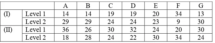
[image:6.595.113.464.522.593.2]This is best done by first calculating the response table for the factors (or interactions) using the frequencies.
Figure 4.2 Response Table of Factor Effect
A B C D E F G
Level 1 14 14 19 19 20 34 13
(I)
Level 2 29 29 24 24 23 9 30
Level 1 36 26 30 32 24 20 30
(II)
Level 2 18 28 24 22 30 34 24
Figure 4.3 Analysis of Variance
Source Pool Sq v Mq F-ratio Sq’ rho %
A Y 0.29 2 0.15 - -
B 15.70 2 7.88 - 10.96 4.41
C Y 0.03 2 0.01 - -
D 41.03 2 20.56 - 31.224 12.36
E Y 0.28 2 0.15 - -
F 13.50 2 6.75 - 11.88 3.72
G Y 0.77 2 0.33 - - -
Pooled e 249.7 249.7 0.80 - 254.6 79.5
5. References
[1] N. Belavendram, Quality by Design, Prentice Hall, 1995.
[2] D.C.Montgomery, Design and Analysis of Experiments, John Wiley & Sons, Singapore,1991