Stability Reserve in Stochastic Linear Systems with
Applications to Power Systems
Humberto Verdejo
Department of Electrical Engineering University of Chile
Luis Vargas
Department of Electrical Engineering University of Chile
Wolfgang Kliemann
Department of Mathematics Iowa State University
Abstract—This paper studies linear systems under sustained random perturbations with the purpose of defining a stochastic stability reserve, i.e., of computing for a given size of the pertubation the values of the system parameters for which the system shows the best stability behavior. The stochastic perturbation model is given by a bounded Markov diffusion process. The Lyapunov exponent is used for computing the stability reserve. This paper presents a short description of four numerical methods for the computation of the Lyapunov exponent and the methodology is applied to linear oscillator in dimension 2 and to a one machine - infinite bus electric power system.
I. INTRODUCTION
In their operation, electric power systems are subjected to a variety of random perturbations, which affect all aspects of system behavior, including small signal analysis as well as contingency studies and transient stability analysis. Basically all probabilistic analysis of power system behavior addresses contingency and security / reliability analyses, see e.g. [10]. Notable exceptions that deal with small signal analysis under random perturbations include, e.g., [8], [9], and [13]. These papers consider systems under white noise excitation and discuss stability criteria ([8] and [9]) or noise-induced chaos ([13]).
In the context of small signal analysis of linearized systems, Lyapunov exponents provide information about the almost sure (exponential) stability of systems under random perturbations, generalizing the real parts of the eigenvalues of determin-istic linear systems. In [12] we presented the theoretical development for computing the Lyapunov exponents of linear stochastic systems. In this paper, we consider perturbations of varying size, and study their impact on the resulting Lyapunov exponents. This allows us to study the stability reserve in such systems.
This paper is organized as follows: In Section II we briefly introduce the model and discuss almost sure Lyapunov expo-nents. Section III presents the model of the perturbation and re-views numerical methods for computing Lyapunov exponents. Section IV describes the two examples for which we present stochastic stability results in Section V.
II. METHODOLOGY
A. Lyapunov Exponents and Stability of Stochastic Linear Systems
Consider the system
˙
x=A(ξt)x inRd, (1)
whereξt is a perturbation process of the following type: Let
dηt=Y0(ηt)dt+ l
X
i=1
Yi(ηt)◦dWt inM (2)
be a stochastic differential equation on a compact C∞
−manifold M with C∞
−vector fields Y0, ..., Yl. Here
”◦” denotes the Stratonovic stochastic differential. We assume that (2) has a unique stationary and ergodic solution with invariant distribution ν on M, which is guaranteed, e.g. by the weak nondegeneracy condition
dimLA {Yi, i= 1, ..., l}(y) = dimM for ally∈M,
(3) where LA denotes the Lie algebra generated by the vector fields Yi. The system perturbation ξt in (1) is modeled as a
function of the background noiseηt in the form
ξt=f(ηt) f :M →U ⊂Rm (4)
with f a C∞
function that is onto a compact set U ⊂ Rm
with 0 ∈intU, the interior ofU. This set-up gives us great flexibility when modeling a (bounded, stationary, Markovian) perturbation of the system.
We denote the solutions of (1) at time t ≥ 0 with initial valuex∈Rdbyϕ(t, x, ξ
t). Their exponential growth behavior
is given the Lyapunov exponents
λ(x, ω) = lim sup
t→∞ 1
t log(kϕ(t, x, ξt(ω))k), (5) whereω is an element of the probability space on which the stochastic differential equation (2) is defined. For background material on Lyapunov exponents of stochastic systems we refer the reader to [1], [4] and [14].
In general, the stochastic system (1) with ergodic perturba-tionξtcan have up toddifferent Lyapunov exponents. Under
a mild nondegeneracy condition on the invariant directions of A(ξt), however, one has a unique exponent with probability 1.
This condition is expressed in terms of the induced system on the sphere inRd: Since the system (1) is linear, its projection
onto the sphereSd−1
⊂Rdis given by the random differential
equation
˙
s=h(A(ξt), s) s∈Sd
−1
(6) h(A, s) = (A−sTAs·I)s
where ”·T” denotes the transpose of a vector, and I is the
d×d identity matrix. We assume the following ’richness’ condition on the background noise (2) andA(η)projected onto the sphere
. With these preparations we have the following result:
Theorem 2.1: Consider the linear system (1) with stochastic perturbation (2,4) under the assumptions (3,7). Then the system has a unique Lyapunov exponent
λ≡λ(x, ω) = lim
t→∞ 1
t log(kϕ(t, x, ξt(ω))k) (8) for allx∈Rd\ {0}, almost surely.
This theorem was first proved in [3], the version presented here follows the set-up of [4]. The Lyapunov exponent from Theorem 2.1 determines the stability behavior of the solutions of (1) in the following way:
Corollary 2.2: Under the conditions of Theorem 2.1, the zero solution ϕ(t,0, ξt) ≡ 0 of the stochastic linear system
˙
x(t) =A(ξt)x(t)is almost surely exponentially stable if and
only ifλ <0.
Theorem 2.1 and Corollary 2.2 are the basis for numerical methods for Lyapunov exponents, which we address in the next section. The setup presented here is quite flexible in the sense that the background noise ηt in (2) allows the modeling of
bounded, stationary perturbations with any rational spectrum (e.g. as projection of an Ornstein-Uhlenbeck process onto a sphere), and hence the system perturbation ξt = f(ηt) can
model stochastic processes with a wide variety of statistical characteristics. Of course, in applications to actual power systems bothηt andf need to be estimated from actual data,
such as variations in generation or loads.
So far we have considered systems with a fixed random perturbation ξt, t ≥ 0. To judge the actual stability reserve
in a system, we study the system response to perturbations of varying size. Keeping the background noise in (2) fixed, we introduce a parameterized family of functions
fρ :M →Uρ⊂Rm, Uρ:=ρU
fρ(η) :=ρ·f(η), ρ≥0.
Recall the requirement that 0 ∈ intU, and hence this setup models varying perturbation ranges. For ρ = 0 we recover the unperturbed system, and forρ= 1 we obtain the system (1). The assumptions (3) and (7) are valid for all ρ > 0 if they hold for ρ = 1. Hence Theorem 2.1 and Corollary 2.2 guarantee the existence of a unique Lyapunov exponentλρ for
all ρ > 0. For the sake of comparison with the unperturbed (deterministic) system we define λ0 to be the maximal real part of the eigenvalues of the system matrixA:=A(ξt= 0).
III. NUMERICALMETHODS
A. Perturbation model
For the case studies in Section IV we use as background noise an Ornstein-Uhlenbeck process
dηt=−ηtdt+dWt inR1. (9)
The system noise is given by
ξt=ρ·sin(ηt), ρ≥0 (10)
resulting on an Ornstein-Uhlenbeck process on the circle S1
with magnitude1.
The stochastic differential equation (9) is solved numer-ically using the Euler scheme, compare [6]. The resulting linear equation (1) and the projected equation (6) are solved numerically using an explicit 4-th order Runge-Kutta scheme.
B. Method 1: Computing the Lyapunov exponent from the linear system
For general background information on the numerical com-putation of Lyapunov exponents we refer the reader to [5], [11], and [14]. is solved on the time interval[0,1], resulting inβ time series xj(n)(i)withn= 0, ..., k. We definexj1(i) :=x
to be the initial condition for the time interval[1,2], and we continue in this way over the time interval[0, T]. For each trajectoryηt(i)of the background
noise and each initial valuexj0we obtain an approximation of the Lyapunov exponent via
λj(i) = 1
Averaging expression (11) over the β realizations of the background noise results in an estimate
λj= 1
of the time-T Lyapunov exponent from the initial valuexj0∈
Sd−1
, and further averaging over the initial conditions gives the estimate
for the time-T Lyapunov exponent of the linear stochastic system (1).
exponent after timeT1 > 0. For T1 ∈N with T1 < T, one obtains instead of (11) the following formula
λj(i) = 1
The other averages are then computed as in (12) and (13).
C. Method 2: Computing the Lyapunov exponent from the projection of the linear system
As in Section III-B we fix a time interval[0, T],T ∈N, a
step sizeh, and we pickαinitial conditions xj0∈Sd
−1
,j = 1, ..., α. The time series of the background noise are computed as in Method 1. In this approach, for each initial condition the linear system (1) is solved for one time steph, and the resulting point inRd is projected onto the sphereSd−1
. Continuing in this way, one obtains a time seriessj
n(i) :=xjn(i)/
xjn(i)
for n= 0, ..., T k. This time series is a numerical approximation of the solution of the projected system (6). Using Formula (13) in [12] we obtain
λj(i) = 1
as the time-T approximation of the Lyapunov exponent for the initial condition xj0 ∈ Sd
−1
and the background trajec-tory ηt(i). For the results in Section IV we have used the
trapezoidal rule to evaluate the integral in (15). Averages over the background trajectories and the initial conditions are now computed as in (12) and (13).
As for Method 1, one often obtains more consistent results when using a burn-in periodT1>0, i.e. by considering
λj(i) = 1
For this method, such burn-in periods are often essential since the expressionsTAsin (15) can take, for some systems such
as realistic power systems, very large values whens∈ Sd−1
is close to one of the axes inRd.
D. Method 3: Computing the Lyapunov exponent from the projected system
This method is the same as Method 2, except that the trajectories sj
n(i) for n = 0, ..., T k on the sphere Sd
−1
are computed directly using the nonlinear differential equation (6) of the projected system. We have used an explicit Runge-Kutta scheme of order 4 for the case studies in Section IV. Within this setup, Formulas (15) and (16) hold without change. When using this method, burn-in periods are essential since the expressionsTAs also appears in the vector field on the right
hand side of (6).
E. Method 4: Invariant distribution on the sphere
Under the conditions of Theorem 2.1 the pair process P
s(t, s0, ξt)
ηt
has a unique stationary distribution µ on
Pd−1×M
with marginal ν on M, compare, e.g., [2]. Here
Pd−1
denotes the projective space ofRd, and this space needs
to be considered sinceϕ(t, αx0, ξt(ω)) =αϕ(t, x0, ξt(ω))for
allα∈R,α6= 0. The mapP :Sd−1
→Pd−1
is the projection, identifying opposite points on the sphere. On Sd−1
×M we either have one stationary distribution (iff the support ofµis all ofPd−1
×M), or two that are reflections at the origin of each other. Letκbe the marginal ofµonPd−1
(or one of its copies on Sd−1
), then the ergodic theorem implies that
λ=
Z
Pd−1
sTAs dκ almost surely. (17)
For lower dimensional systems, Formula (17) often provides a convenient way to compute the a.s.Lyapunov exponent of a linear system, compare the discussion in [14]. For higher dimensional systems, such as power systems, the reliable computation of the density of κ is prohibitive in terms com-putation time and data storage. Therefore, we do not pursue this approach in the current study.
We have tested all four methods for a variety of systems, compare e.g. the results in [12], and we have chosen Method 1 for this paper because of its accuracy and speed.
IV. EXAMPLES
A. Two-dimensional linear oscillator
˙
x+ 2by˙+ (1 +ξt)y= 0 (18)
or in the state space form
˙
The key parameter of the linear oscillator is the damping b, for which we chose values b ∈[0,3]. For the range of the random perturbation we used ρ∈[0,4], in increments of 0.2. The results in Section V were produced with a numberβ = 60
of realizations, and a number α = 41 of initial conditions, spaced uniformly.
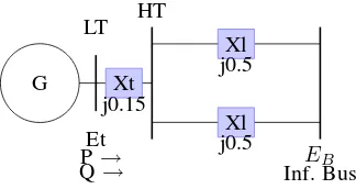
B. One machine-infinite bus power system
In the area of power systems, we present the classical example of a one machine-infinite bus system, compare [7].
G Xt
We use the following parameters
P= 0.9(p.u) Q= 0.3(p.u) (overexcited)
˙
Et= (1.0∠36o) E˙B = (0.995∠0o).
The state vector for the linear system∆ ˙x=A∆x, is
∆x= [∆ω,∆δ,∆Ψf d, v1, v2, v3] (19) where v1, v2, v3 are variables of the PSS, using expressions defined in [7]. The matrixAhas the structure
A=
a11 a12 a13 0 0 0 a21 0 0 0 0 0
0 a32 a33 a34 0 a36
0 a42 a43 a44 0 0 a51 a52 a53 0 a55 0 a61 a62 a63 0 a65 a66
and the differential equation for the field circuit is:
∆Ψf d=
K3
1 +sT3
(∆Ef d−K4∆δ), (20) with excitation system
∆Ef d=−KA∆v1, (21) wherev1 is the output of the voltage transductor. The pertur-bation has been introduced as affecting the reference signal. This situation is described by changing the elementa34 in the matrix A to
∆Ef d=−KA(1 +ξt)∆v1. (22) In this section we consider the (linearized) one machine -infinite bus systemx˙ =Axwith system matrix
A=
0 −0.11 −0.12 0 0 0
377 0 0 0 0 0
0 −0.19 −0.42 −27.4 0 27.4
0 −7.3 20.8 −50 0 0
0 −1 −1.1 0 −0.71 0
0 −4.8 −5.4 0 26.9 −30.3
,
where a3,4 = a3,4·(1 +ξt) is a stochastic perturbation as
described above. The stochastic perturbation isξt=ρ·sin(ηt)
withηtan Ornstein-Uhlenbeck process as in (9).
The key parameter in this system is the gain of the PSS, KP SS, whose nominal values was chosen as in [7]. To study
the stability reserve of this system, we used gain valuesKγ:=
γ·KP SS, withγ= 0.5,1,5,10,15,20,25. For the range of the
random perturbation we usedρ∈[0,4], with a step size of0.2. The results in Section V were produced with a numberβ= 30
of realizations, and a number α = 54 of initial conditions, spaced uniformly on a regular grid in(∆δ,∆ω)−space (angle, angular velocity).
The time of simulation for the results in Section V isT = 30sec. We tested the system also with T = 60sec and T = 90sec, and obtained similar results.
V. RESULTS
A. Example 1: The linear oscillator
(a) Lyapunov Exponents
(b) Level curves
Fig. 2: Two-dimensional linear oscillator
Figure 2a shows the almost sure Lyapunov exponentλρ(b)
depending on two parameters, the perturbation sizeρand the damping b. Figure 2b contains the different levels curves of the surface in Figure 2a. These figures show two important results:
1) For a fixed value b0 ≤ 1 of the damping, the a.s. Lyapunov exponentλρ(b
0)grows in a monotone fashion with the perturbation size ρ, while for b0 > 1 the exponentλρ(b
2) For the unperturbed system (withρ= 0) the Lyapunov exponent is at its minimum forb= 1, withλ0(1) =−1. For a fixed value ρ0 >0 of the perturbation range, the behavior is similar, except that the value b(ρ0) of the damping, at which the minimal Lyapunov exponent is realized, increases with increasing perturbation rangeρ. These two observations allow us to determine, for each perturbation sizeρ≥0, the damping valueb(ρ)at which the stability reserve of the system is maximal, i.e. at which the Lyapunov exponentλρ(b)is minimal.
B. Example 2: One machine - infinite bus system, Part I
(a) Lyapunov Exponents
(b) Level curves
Fig. 3: One machine-infinite bus power system with huge values
Figure 3a shows the almost sure Lyapunov exponentλρ(γ)
depending on two parameters, the perturbation sizeρand the factorγ determining the PSS gainKγ as described in Section
IV-B. Figure 3b contains the different levels curves of the surface in Figure 3a. Note that in this example the range of the PSS gain is very large, up to25times of the nominal value KP SS.
This example shows basically the same qualitative behavior as Example V-A. The only difference is that for small pertur-bation rangesρthe optimal PSS gainγ(ρ)is somewhat smaller than the optimal deterministic value. But for larger ρwe see the same behavior as before: The optimal stability reserve of the system is attained for gain factorsγ(ρ)that are larger than the optimal deterministic valueγ0= 10.
C. Example 3: One machine - infinite bus system, Part II
(a) Lyapunov Exponents
(b) Level curves
Fig. 4: One machine-infinite bus power system with tipical values
In this example we have considered the one machine -infinite bus system from Example V-B for PSS gains that are close to the nominal value KP SS, i.e. for values of γ in the
range γ ∈ [0,1.4]. Figures 4a and 4b show a more detailed picture of lower ranges in Figures 3a and 3b. As expected, for fixed ρ > 0 the Lyapunov exponent λρ(γ) is basically
of gain factors hardly affects the stochastic stability reserve of the system.
VI. CONCLUSION
In this paper we have analyzed the stability reserve of a lin-ear stochastic system using almost sure Lyapunov exponents. The idea is to compute the exponentλρ(p)for various values
of the perturbation range ρ ≥ 0 and of the tunable system parameter(s)p. The computed surface ofλρ(p)allows us, for
each noise range, to obtain the optimal tuning valuep(ρ) for the parameter, resulting in maximal stability reserve for this noise level. We studied the case of the linear oscillator (with damping coefficientbas the tuning parameter) and of the one machine - infinite bus power system (with PSS gain constant as the tuning parameter). In both cases the optimal tuning value under random perturbations is larger than the optimal value of the unperturbed (deterministic) system. However, if we restrict the PSS gain to a small neighborhood of its nominal value, the λρ(p) level curves are basically flat, i.e. the PSS gain in
this range does not have much of an effect on the stochastic stability reserve of the system.
ACKNOWLEDGMENT
This work was supported by The Institute of Complex Engineering System, by Mecesup (Project FSM0601) and BECAS-CHILE program.
REFERENCES
[1] Arnold, L., Random Dynamical Systems, Springer-Verlag, 1998. [2] Arnold, L. and W. Kliemann, On unique ergodicity for degenerate
diffusions, Stochastics 21 (1987), 41-61.
[3] Arnold, L., W. Kliemann, and E. Oeljeklaus, Lyapunov exponents of linear stochastic systems, Springer Lecture Notes in Mathematics No. 1186 (1986), 85-125.
[4] Colonius, F. and W. Kliemann, Spectral theory for perturbed systems, GAMM Mitteilungen 32,1 (2009), 26-46.
[5] A. Grorud and D. Talay, Approximation of Lyapunov exponents of nonlinear stochastic differential equations, SIAM Journal on Applied Mathematics, 56(2), (1996), 627-650.
[6] Kloeden, P. and E. Platen, Numerical Solution of Stochastic Differential Equations, Springer-Verlag, 2000.
[7] Kundur, P., Power System Stability and Control, McGraw-Hill, reprinted edition, 1994.
[8] Loparo, K.A. and G.L. Blankenship, A probabilistic mechanism for small disturbance instabilities in electric power systems, IEEE Transactions on Circuits and Systems 32 (1985), 177-184.
[9] Namachachivaya, N.S., M. A. Pai, and M. Doyle, Stochastic approach to small disturbance stability in power systems, in: Lyapunov Expo-nents,(Arnold, L., H. Crauel, and J.-P. Eckmann, eds.), Springer Verlag, (1991), 292-308.
[10] Schilling, M.T., R. Billinton, and M. Groetaers dos Santos, Bibliography on power systems probabilistic security analysis 1968-2008, International Journal of Emerging Electric Power Systems 10 (2009), 1-48. [11] Talay, D., Approximation of upper Lyapunov exponents of bilinear
stochastic differential systems, SIAM Journal on Numerical Analysis, 28(4), (1991), 1141-1164.
[12] Verdejo, H., L. Vargas, and W. Kliemann. Stability of linear stochastic systems via Lyapunov exponents and applications to power systems, submitted to IEEE Transactions on Power Systems.
[13] Wei, D.Q. and X.S. Luo, Noise-induced chaos in single-machine infinite-bus power systems, Europhysics Letters 86 (2009), 6pp.
[14] Xie, W.-C., Dynamic Stability of Structures, Cambridge University Press, 2006.