sc
ACSIS 2012
ISBN: 978-979-1421-15-7
zyxwvutsrqponmlkjihgfedcbaZYXWVUTSRQPONMLKJIHGFEDCBA
A n Im plem entation
of F uzzy Inference System for
O nset P rediction B ased on Southern O scillation Index
for Increasing the R esilience of R ice P roduction
A gainst C lim ate V ariability
.
Agus Buono!.
2and Mushthofa'
I)Centt'r for Climate Risks and Opportunity Management in Southeast Asia and Pacific
(CCROM-SEAP) Bogor Agriculture University, Bogor-West Java, Indonesia
zyxwvutsrqponmlkjihgfedcbaZYXWVUTSRQPONMLKJIHGFEDCBA
2)
Department of Computer Sciences, Faculty of Mathematics and Natural Sciences, Bogor
Agricultural University, Bogor-West Java, Indonesia
Email: [email protected]@yahoo.com
zyxwvutsrqponmlkjihgfedcbaZYXWVUTSRQPONMLKJIHGFEDCBA
Abstruct-Riee production system in lndonesia is very sensitive to global phenomena, especially the El Nino phenomenon. Information regarding the onset of rainy season is important to increase the resilience of the production system. This paper is focused on the implementation of Fuzzy lnfcrence System (FIS) as a technique for predieting the onset of rainy season based on the Southern Oscillation Index (SOl) data in the months of' July, August, September and Octobcr. There are two data seh uscd: the 501 data from the year 1877 to 2011 and the rainy scason onset in the District of Indramayu. Fuzzy set memberships and the set of rulcs are deslgned by lnvesttgatlng the two sets of data (via visualization and c1ustering). The prediction system is vcrlfled by using the actual data from the district. The result of the verjfication shows that the corrclation bctwecn the rainy onsct and its predictcd value is 0.68. Even though the prediction accuracy is relativcly cornpctltive comparcd to the existing methods, the requirement of the use of the SOl variablcs from the month of October renders the model less useful in practice, since it would be mostly too late to wait until October to pcrforrn the predietion. Further research can be developcd which lntcgratcs Markov Chain method to ovcrcome this problem.
Index Terms-e- Rice production system, El Nino, Fuzzy lnfcrcnce System, Onsct, Southern Oscillation Index.
-
I. INTRODUCTIONT
he agriculturalsector,
especially the food subsector is one of the important subsectors which is very susceptible toweather and climate change. This is due to the fact that plants generally need a certain clirnate/weather condition based on
empirical data. the variability of rice production correlates strongly to the variability of rain fall. According to [IJ. 81%of crop failures are caused by etimate variabiliry, while only 19% of them are caused by pests. Of the failures caused by etimate variability. 90% are caused by drought occurring during the
second planting season.
Empirical records show that droughts are gencrally
influenced by global phenomena, such as the El Nino Southern Oscillation (ENSO), and by cIimate variables such as: the amount of rainfall, the Iength of the rainy season, as well as the
onset of the rai ny season. Therefore, early information regarding these c1imate variables can be very useful in determining anticipative steps in rice field cultivation,
This paper specifically presents an implementation of a Fuzzy Inference System for the prediction of rainy season
onset, Buono, et. al. (2012), [2] has developed an artificial neural network model based on SOl data on the rnonth of June, July and August. The resulting accuracy was not so satisfactory. of about 0.6. Also, the model was built using data only from one station, so that the model could not represent the general characteristics of a certain area. In this research. a fuzzy system is developed based on the knowledge gained
from data exploration in a certain district to cover a larger range of area. Also, the computation of the output from the input data is based on a logicai knowledge backed by observation data. Accordingly, it is expected to have a better accuracy result than the previous research.
The remainder of this paper is organizcd as follows: Section 2 presents the principles of rice production in Indonesia. Section 3 describes the data and the methods, Scction 4 is addressed to explain the design of the computational model.
Results and discussions are presented in Section 5, and final ly, Section 6 is dedicated to the concIusions of this research study and recommendations for future research.
II. RICE PRODUCTION SYSTEM
In general, for Indonesian farmers there are two planting season: ramy season and dry season. On the first season. planting begins during the start of the rainy season and continues for the next four months. For fields located near the inigation channels, planting can be immediately done. For
fields located farther away from the channels, however, planting will be delayed in accordance to their distance from the irrigation channcls. This kind of planting pattem will be
ICACSIS 2012
continuously affected by the characteristics of the c1imate, be it normal, or in the presence of El Nino or La Nina, as depicted
in Figure 1.
450
zyxwvutsrqponmlkjihgfedcbaZYXWVUTSRQPONMLKJIHGFEDCBA
1
~
'"
350s
:s
.
300•
2SO<
e,li
200zyxwvutsrqponmlkjihgfedcbaZYXWVUTSRQPONMLKJIHGFEDCBAI..
150 Ia I
~
;.
100 .'
:
50
...
: 09 10 11 12
-4--00"'"
•••• , •• B p4ro
- oo- -U 1ft!
t
:'"--Q\···
..'.
'.
zyxwvutsrqponmlkjihgfedcbaZYXWVUTSRQPONMLKJIHGFEDCBA
'. 0 ,....
, -0, ' '0
O
'b... ',,' \.
-
~
6 a
[image:2.599.71.276.139.279.2]Month
Figure I. Yearly planting pattem accord ing to the three clirnate conditions (Source: [3])
It
can be seen from the picture that the peak of planting will experience delay in the presence El Nino, and experience advancement in the presence of La Nina. Problerns often rise during the presence of El Nino, especially for the secondplanting (dry season). Rice production during this second plant ing will be highly susceptible to drought, especially for areas farther from irrigation channels. On these areas, the first planting cannot be performed in the beginning of rainy season. Therefore, the second planting will also be delayed, so that the risk of facing drought will be higher. By having the predictive information regarding the onset of rainy season, anticipative steps can be taken to prevent greater losses.
III. DATA AND METHOD
zyxwvutsrqponmlkjihgfedcbaZYXWVUTSRQPONMLKJIHGFEDCBA
A. Data
The first data used for this research is the Southern Oscillation Index data, which can be downloaded at http://www.bom.gov.aulclimate/currentlsoihtml.shtml. From this site, we collect the monthly SOl Index from the year 1877
to 2011. The second data prepared is the observational data of
the onset of the rainy season obtained from live rainfall zones in the District of Indramayu. From each zone, we collect the onset of rainy season data from the year 1965 to 2009, with a few missing values.
The SOl index is the difference between the anomaly of the air-pressure in the Tahiti region and the Darwin region, divided by the standard deviation of the differences. and written as: [4]
SOl Index
=AlIP(Tahili)
- AnP(Danl"in)
x10
(I)STD(Diff)
with:
AnP(Tahiti) Anl'(Darwin)
STD(DifJ)
=
Tahiti air-pressure anornaly =Darwin air-pressure anomaly = The standard devi at ion of thebetween the above variables
difTercnces
15I30:: 9,S-979-U21-15-7
Stone (1996) shows that SOl index (which is a global phenomenon) has intluences on local c1imate condition,
especially in Indonesia. Generally. there are live conditions on
the values of 501 index, known as the 501 Phases, which are determined based on the values of 501 from two consecutive
months, as shown in Figure 2.
..
RAPIDPhase Q FALL .ee
f.
~
[image:2.599.332.547.168.320.2].>0 7
Figure 2. Fivc 501 Phascs based on the SOl values ottwo consccutive months
(Sourcc.] 4 Jl
Based on crnpirical data. rt the S01 talis IIHO Phase ior.3 then there is a tcndcncy towards the prcscncc of El Nino.
Meanwhile, La Nina isgenerally preceded by 501 Phase 2or
4. If501 is in Phase 5,it is generally expccted that the climate
will run in a normal course.
The data for the onset of rainy season is measured within a period of 10 days. Hcnce. there are 36 possible values of rainy scason onset: from 1 (first ten days of the year) to 36 (the last
10days of a year. one year is approx imated to be 360 year. As
an cxamplc. if the onset value is 33. then this mcans the start
of the rainy season is around the last week of November. We follow the definition of rainy xeason onsct according to Moron
r
51· which is: the occurrence of min above 501ll1ll during 3 consecutive lOvday periods. Ba-ed on the data from 191i5 102009. the avcrage onset <1110111<111' in the district of Indramayu is as presented in Figure 3. Negative values mean rainy season occurred ahead of normal. \\ hill' positive values mean tha: ril lilY -cason occurrcd [ater than norma I.
A.nomaly of Onset
'".
F1gllr~ -' The ;HlnI11JI~ paucrn tlrraln~ "t.::l'.•OT1onvct dara ln lndramavu from
IfI(" 1%(, Ip cOO!):Olfl
ICACSIS 2012
zyxwvutsrqponmlkjihgfedcbaZYXWVUTSRQPONMLKJIHGFEDCBA
B. M ethod
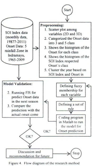
The development of the flS model in this research follows the steps outlined at figure 4.
a. Data Exploration: ln this step, data exploration is performed
inorder to obtain knowledge on two things: the distribution pattern of the SOl and the pattem of the relationship between SOl with the onset. The information regarding the distribution pattern of the SOl and the rainy season onset is
used to determine the fuzzy sets of these variables, while the pattern of the relationships between the SOl and the rainy season onset data is used to determine inference rules mapping input variabie (SOl) to output variable (rainy season onset).
b. Fuzzyfication: On this step, we define the fuzzy sets for each of the variables, namely: the SOl and the rainy season onset. ln this case, the rainy season onset values are represented as the values of the anomaly of the onset, obtained from the original values of the onset, subtracted by their mean, computed from the data obtai ned from 1965 to 20 JO.
c. Rule Generation: On this step, rules are constructed which maps the input variable to the output variable. Other than the use of the relationship pattern between the SOl and the rainy season onset, the construction of the rule also uses c1usters analysis. In this case, we perfonn year clustering based on the values of the SOl variable to find the c1usters of the SOl data. Based on this c1uster analysis, we characterize the onset values and deterrnine the fuzzy inference rules. d.lmplementation and evaluation: on this step, an
implementation program is written using the Matlab programming language to build the fuzzy inference system. Evaluation is performed by computing the output of the system when supplied with the available data, and companng the results against the available rainy season onset data.
IV. MODEL DESIGN
zyxwvutsrqponmlkjihgfedcbaZYXWVUTSRQPONMLKJIHGFEDCBA
A. SOlllldex and Onset Data Exploration
Here we perform visual data exploration with the purpose of obtaining the characteristics of SOl. and the relationship
berween the SOl and thezyxwvutsrqponmlkjihgfedcbaZYXWVUTSRQPONMLKJIHGFEDCBAonset values. The onset values are
divided into three categories. namely: delayed, represented by
the value I) normal (represented by the value 0) and early onset (represented by the value -I ).
These categories are based on the anomaly of the onset values obtained from 1965 to 2009, computed from the mean value of 33. For an example. consider that in the year
2002/2003. the onset value was 35. hence the anomaly is
35-33 =2. categorized as the value 1 (delayed). This will make it
casicr to noticc the relationship between the SOl and onset values. We will first examine the distribution pattern the SOl. and followed by the relationship pattem berween the SOl and the on et values.
ISBN: 978-979-1421-15-7
Model Vali<btion:
2. Running FIS for predict Onset data in the next season 3. Com pare the
prediction with the actual onset come
Preproeessing: I. Scatter piot among
variables (2Dand3D)
2. Categorized the Onset data into 3and 5class 3. Shows the bistogram of the
Onsct for each class
4. Shows the histogram of the SOl Index respected Onset s el ass
5. Cluster the year based on SOllndex and Onset in
[image:3.599.332.526.78.427.2]Onsct prediclion
Figure 4. Flow diagram of the research method
;
, ,
"-lC I.
,
I')SOl>..,
Figure 5 shows the distribution pattem of the SOl in the
months of July to October (Red: delay. black: normal, green: early). From Figure 5, we can conclude that for early onset,
the distribution of the SOl values tend to be positive with a mean value of approximately 7.5. This occurs on each of the four months. On the other hand, for normal and delayed onset
values in the month of July shows a small difference. However for the month of August September and October, the differences are significant, despite still be smaller than in the early Onset.
\
I'
\
-
,,~--Ju 10
-- -...:.-...
I. 10
zyxwvutsrqponmlkjihgfedcbaZYXWVUTSRQPONMLKJIHGFEDCBA
~ - --- --- · 1
I
(]
I
I
.1
i '
ok...- ~ o~
zyxwvutsrqponmlkjihgfedcbaZYXWVUTSRQPONMLKJIHGFEDCBA
~ 1 0 0 1 0 ~
sot_5e9
297
1,
,.
---
2'0 10 0 11'1soi.oe
ICACSIS 2012
The average SOl for early delayed and normal onset for the months of August, September and October are relatively equal,
with each ranges approximately -7.5 and
o.
The average for July in normal onset is about -2.5, while for delayed onset is approximately -5. On top of that, to further increase the sensitivity of the system, 5 memberships sets for SOl aredefined: Very Negative, Negative, Zero, Positive and Very
Positive. The complete membership functions for SOl are
given in Figure 6.
zyxwvutsrqponmlkjihgfedcbaZYXWVUTSRQPONMLKJIHGFEDCBA
J.l(50I Index)
FigurezyxwvutsrqponmlkjihgfedcbaZYXWVUTSRQPONMLKJIHGFEDCBA6. Fuzzy membership for SOl Index
On the other hand, there are five pattems of the rainy sea son onset data, as given in Figure 7. From Figure 7, itcan be seen that the centers of the clusters of the onset anomaly are: approx. -3.2, -1.5, 0, 1.7and 3.5. Based on this information,
the fuzzy sets for the onset values are constructed as presented
in Figure 8.
zyxwvutsrqponmlkjihgfedcbaZYXWVUTSRQPONMLKJIHGFEDCBA
B. Building the Set ofInference Ril/es
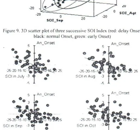
Figure 9 shows the distribution of data points in 3D of the three SOl values. From this figure, we can see a clear relationship between the SOl values and the onset values. In this case, if the SOl value is negative, then the onset anornaly
tends to be positive (red), which means that the rainy season
onset is likely to be late. On the other hand, positive SOl values indicates that the rainy season onset will tend to be negative, which means that rainy season is likely to be ahcad of normal.
16
14
12
•.
10II
l!
f
8t 6
4
i
2 I
J
0--4 · 2 0
An_Onset
,,-
Sto.-."
· uu 0.5001 1 · Ut· 0."312 11
00.0"" O.S012 II
zyxwvutsrqponmlkjihgfedcbaZYXWVUTSRQPONMLKJIHGFEDCBA
I.JOJ O.Sl1; !
J.4S5 O.~
•
4
Figure 7. The Distribution pattem of the rainy season onset
ISBN: 978-979-1421-15-7
.u(Onset .4nomaly)
Onset An. is
VeryNegative
Onset is An.
VeryPositive
-5.5 -4 -2 -1
o
2 45.)
[image:4.599.316.557.93.248.2]Onset Anomaly
Figure 8. Fuzzy membership for the Onset Anornaly
This relationship appears to be consistent from July to August. These facts are also back ed by the scatter piot Jn Figure 10.
•
•
20
[image:4.599.322.554.398.614.2]·20
Figure 9. 3D scatter pIot of three successivc SOl Index (red: delay Onset. black: normal Onset, green: early Onset)
.'i
SOllnSep ·3
.~
Figure 10.20 Scatter piotbcrwccn SOl Index with Anomaly ofOnset
Based in these two facts, it is fairly logicai to use the SOl to predict the value of the rainy season onset. We can also conclude that if the SOl value decreases, then the onset anomaly value should increases. which means that the rainy season will be delayed. The onset anornaly will be normal when the 501 is in the Zero Phase. Finally. a positive value of the SOl will lead to negative onset anomaly, which rneans that the rainy season onsct is delayed. To obtain other possible patterns. we perfonned cluster analysis using the SOl variable and the onset anomaly variable.
ICACSIS 2012
-290.38zyxwvutsrqponmlkjihgfedcbaZYXWVUTSRQPONMLKJIHGFEDCBA
f
-160.25-30.13
zyxwvutsrqponmlkjihgfedcbaZYXWVUTSRQPONMLKJIHGFEDCBA
1 0 0 . 0 0 ,
.•.~~~'\..~~~~~'''~'i'
[image:5.597.323.541.75.163.2]Observatlons
Figure II. Dendrogram showing the result of the year c1usteringbased on the
SOl andthe onset
Figure 11 shows the dendrogram of the cluster analysis on the year 1965 to 2009. By cutting the dendrogram on Figure
II along the dashed line, we obtain 8 clusters which
correspond to 8 fuzzy rules. The average values of the SOl and onset anomaly for the 8 clusters are presented in Table I. From Table I, we can create 8 different fuzzy rules, namely:
Rule I: IFzyxwvutsrqponmlkjihgfedcbaZYXWVUTSRQPONMLKJIHGFEDCBA(501
zyxwvutsrqponmlkjihgfedcbaZYXWVUTSRQPONMLKJIHGFEDCBA
in Ju~1'is Ven' Negativei and (501 in August is VeryNegative) and (501 in September is VeryN egativei and (501
in October is Very Negative)
TH EN (Onset Anomaly is Very Positive)
Rule 2: IF(501 inJuly is Zero) and (501 in August is Positive) and
(501 in September is Zero) and (501 inO ctober is Zero)
TH EN iOnset Anomalv is Negative';
Rule 3: IF (501 inJuly is Negative'[ and (501 in August is Zero) and
(501 in September is Positive) and (501 in Deta ber is
Positive)
TH EN (OllSetAnom aly is Positive)
Rule 4: IF (501 inJulv is Zero) and (501 in August is Positive) and
(501 in September is Very Positive) and (501 in Oetober is
Very Positive)
THEN (Onset Anomalv is Zem)
Rule 5: IF(501 inJuly is Negative) and (SOl in August is Negativei
and (501 in September is Negativev and (501 in O ctober is Negauvet
TifEN (Omet Anom aly is Zem)
Rule 6: IF (501 in JI/ly is VelY Positivei and (501 in August is Very'
Positivet and (501 in September is Very Positivei and (501
in Deta ber is Very' Positive)
THEN (Onset Anom aly is I'en' Negative;
Rule 7: IF (501 in JI/Ir is Zero) and (501 inAugust is Zero) and (501
in September is Zero) and (501 in Deta ber is Negativei
THEN (Onset Anomalv is Positive)
Rule R: IF (501 in JI/ly is Zero) and (501 in August i.' Negativev and
(501 in September is Zero) and (501 inO ctober isPositive';
TU ENiOnset Anomalv is Zero)
Table I. Average SOl Index and Onsct Anomaly for each clustcr
Cluster SOllndn in Onset
Jul. Aug. S~p. Oct. Ano. -14.20 -14.00 -14.76 ·1~.60 2119
2.73 3.23 1.36 -0.83 -133
ISEN: 978-979-1421-15-7
Cluster SOl Index in Onset
Ju!. Aug_ Sep. Oct. Ano.
3 -5.00 2.85 7.50 8.55 2.79
4 -0.32 7.88 12.58 11.90 -0.37
5 -10.43 -10.98 -9.36 -8.80 0.38 6 13.50 12.48 16.30 13.63 -2.20
7 3.90 -2.00 -0.04 -8.32 1.29
8 2.20 -6.85 1.55 5.73 -0.74
The fuzzy inference model used in this research is the
[image:5.597.50.295.84.246.2]Mamdani-type inference using centroid as the defuzzification method. The structure of the model is as presented in Figure 12 [6].
Figure 12. The structure ofthe F1S with 8 rules.
V. RESUL T AND DISCUSSIONS
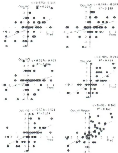
ln order 10validate the FIS that has been developed by using
Matlab, we predict the Onset of 5 rainfall Zones in Indramayu
and their average (also caI led district level Onsets). Scatter
pIot between the actual Onsets with their predictions for 5
rainfall zones and the district level are depicted by Figure 13.
.,~09S. OH\
(lb\.W' ,1.0219.
..
-
•
• •
..
,
J " ___~T--:l J •Pr!!'d Pre-d
•
•
j•
•
•
•
•.
,
-I" 0 78<",. o7U.
Oh. VJ3 '(.0 lU.·0.&05 0'-" 'N< R'.,0114 R' ~ ~Q6
W,"
)
•
••
•
•
•
-
.-•
-
• ·-ti..
-
.
.-.;...
•
-
•
'.
•
J ,'.
'
•• :- ) I
•
•
r-eo 0' .••• P· .(J•
• •
•
-.00;.-:h -0 ~]l P; - 0 'bl
•
•
•
•
•
•
•
•
•
"
~
•
..
-,.> ...•••
'.,
/-
...
~
..
...
'
1 ,
~,
..Jo<
•
[image:5.597.353.519.224.364.2]•
[image:5.597.328.530.474.735.2]ICACSIS 2012
Based on figure 13, tV{Oobservations can be made. firstly, that in general, the two series (prediction and actual Onset) have similar patterns, especially for the district level. The correlation is in the range of 0.31 up to 0.65, and 0.68 for the district level. Second ly,
it
seems that other variables arerequired as predictors in the Onset prediction.
Figure
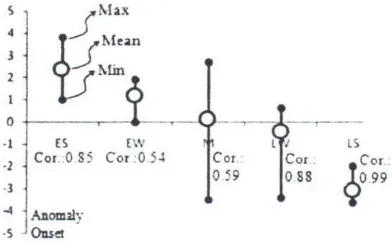
zyxwvutsrqponmlkjihgfedcbaZYXWVUTSRQPONMLKJIHGFEDCBA
14presents the comparison on onset prediction value among ENSO condition (ES:Strong El Nino, EW:EI NinoWeak, M:Moderate, LW:La Nina Weak, and LS:La Nina Strong). IIcan be seen that the Onset resulted by the model are relevant to what c1imatologists would say in real life conditions: that the Onset will come earl; in La Nina and will be delayed in El Nino condition. The magnitude of the anomaly will vary with respect to the level of the ENSO condition. ln addition, we can see that in the moderate condition, the accuracy of Onset prediction drops. This statement is supported by figure 14, i.e. the correlation between the actual rainy onset and its predicted value is 0.59. ln astrong ENSO, the correlation is greater than 0.85. This rneans that, we have to improve the rule and fuzzy rnemberships, and have to explore more detaiis regarding the phenomena in moderate ENSO conditions.
D~;:~
o
+-_v_~r._1in_L
· 1 ·2 · 3
-4 Anom2ly
-s Oeset
t.S
!~or
<;099
ES [W
[image:6.599.81.277.346.470.2]Cor.:0.85 Cor :0.5.l
Figure 14. Comparison prediction ofOnsct Anomaly among ENSO condition
VI. CONCLUSIONS
Based on the experirnent, we can conclude the followings:
a. fuzzy Inference System can be implemented to Onset prediction with an accuracy level of 0.68 in the district level, is able to model and explain them logically.
b. ln strong ENSO condition. the Onset value is easier to predict with higher accuracy compared to the moderate condition.
c. Other predictors are required in order to improve the accuracy.
ln order to increase the system accuracy. for future research we will focus on the parameter optimization of the model and
adding the predictor variable with other ENSO parameters,
zyxwvutsrqponmlkjihgfedcbaZYXWVUTSRQPONMLKJIHGFEDCBA
ACKNOWLEfXiM E)I.'T
This research is funded by I-MHERE Project under contract number: 7/13.24.4/SPP/I-MHEREf2012 Bogor Agricultural University. and partly supported by thc Computer Science Department. Bogor Agriculturc University.
ISBN: 978-979-1421-15-7
REFERENCES
[I] Boer, R. and Perdinan. 2008. Adaptation to climate variability and elimate change: iIS socio-econornic aspect. Proceeding of Workshop on 'Climate Change: lmpacts, Adaptarion. and Policy in South East Asia. Economy and Environmental Program for South east Asia. Bali. [2) Buono, A. A. Kurniawan, and A. Faqih. 2012. The Onset Prediction
by Using Artifieial Neural Network Backpropagation Levenberg-Marquardtet. National Conference: The Application of Information Technology 2012 (SNATI2012), ISSN 1907-5022, Jogyakarta. [3) Boer, R., A. Buono, and Suciantini. 2010. Dynamic Cropping CaJendar
as a Tool to Decide the Cropping Pattern that Appropriate with the Clirnate Condition. I-MHERE Research Report, Bogor Agriculture University.
[4) Stone, R.C", Graeme LM., and T. Marcussen. 1996. Prediction of Global Rainfall Probabilities Using Phases of the Southern Oscillation Index. Nature, Vol. 384,21 November 1996. Nature Publishing Group. [5] ---.2011. Buleting Prakiraan Musim Kemarau 2011, BMKG Semarang. btt,,:llindex.bmk&iateng.comlPRAMK201100f, Accessed on September. 18th. 2012.
[6] Jang J-S R. 2001.
![Figure 2. Fivc 501 Phascs based on the SOl values ottwoconsccutivemonths(Sourcc.]4Jl](https://thumb-ap.123doks.com/thumbv2/123dok/965877.395599/2.599.332.547.168.320/figure-fivc-phascs-based-sol-values-ottwoconsccutivemonths-sourcc.webp)