DOI: 10.12928/TELKOMNIKA.v14i3.2712 916
Distributed Clustering Based on Node Density and
Distance in Wireless Sensor Networks
Sasikumar P1, Shankar T2, Sibaram Khara3
SENSE, VIT University, Vellore, Tamil Nadu – 632 014, India
*Corresponding author, email: [email protected], [email protected], [email protected]
Abstract
Wireless Sensor Networks (WSNs) are special type of network with sensing and monitoring the physical parameters with the property of autonomous in nature. To implement this autonomy and network management the common method used is hierarchical clustering. Hierarchical clustering helps for ease access to data collection and forwarding the same to the base station. The proposed Distributed Self-organizing Load Balancing Clustering Algorithm (DSLBCA) for WSNs designed considering the parameters of neighbor distance, residual energy, and node density. The validity of the DSLBCA has been shown by comparing the network lifetime and energy dissipation with Low Energy Adaptive Clustering Hierarchy (LEACH), and Hybrid Energy Efficient Distributed Clustering (HEED). The proposed algorithm shows improved result in enhancing the life time of the network in both stationary and mobile environment.
Keywords:wireless sensor network, clustering, distributed computing, node density, distance
Copyright © 2016 Universitas Ahmad Dahlan. All rights reserved.
1. Introduction
A WSN of randomly deployed self-operable sensor nodes to monitor physical conditions of the environment, as thermal, acoustic, imaging, etc., as measurements, and collaboratively work together to take the data sensed to the base station. WSNs were originally deployed in military, heavy industrial applications and, later extended to the lighter applications such as consumer WSN applications [1-6].
WSN devices are battery operated; saving power is the biggest challenge. Many work in this area of energy saving have shown that energy is consumed in sensing and monitoring the surrounding area as compared to the data packet exchange activities [1]. Excluding, energy consumption in the nodes such as forwarding nodes and gateway nodes in cluster are higher than other sensing nodes in the cluster. The dynamic topology reformation algorithm method [1] is expected to reduce and balance the energy consumption in WSN. The main purpose of deploying these gateway nodes is to share and balance the energy consumption for demanding jobs in the network.
The battery operated nodes have its own limitation with the respect to the distance it can communicate. Hence they can’t directly communicate to the base station, looking for intermediate nodes to share link. The idea of hierarchical architecture is used to help these nodes by introducing multihop communication strategy. In the later part the clustering algorithms are focussed to give additional features to the multihop communication such as dynamic network management and, data collection and forwarding with limited contention. These features motivated to propose a new clustering algorithm to study the Distributed and Self-organizing Load Balancing Clustering for WSN. The most important issue considered when planning WSN Cluster is the energy consumption per node and how the next protocol can improve this. By switching node activities the power consumed is optimized leads to the increased network life time [1].
2. Related Work
Many clustering algorithms have been proposed considering the distributed processing and direct transmission from Cluster Head (CH) to base station like LEACH, HEED. Thus if the distance between the base station and the cluster head is large then large amount of energy is consumed to send the data to the base station [3]. The above mentioned algorithm uses multi-hop propagation, increases energy conservation. With multi-multi-hop clustering, a link is established between the multiple cluster head nodes like chain and these CH’s work together collaboratively to forward the sensed data by the neighbor nodes in the group to the base station. This multi-clustering mechanism is able to balance the energy consumption among all sensor nodes and achieves an obvious improvement on the network lifetime [3]. Energy-Aware Multilevel Clustering (EAMC) [3] has the following salient features. It aims in reducing the number of cluster heads as cluster heads consume more energy thus less the number of CHs more is the lifetime of the WSN. EAMC forms clustering tree to reduce the amount of relay nodes further ending up in reduced amount of data transmission, shows adaptive nature in addition and removal of nodes into the clusters resulting in robustness of the algorithm.
A robust cluster head selection is important, so that cluster heads spend less energy on aggregating and forwarding messages, doing general route maintenance and some other similar actions. We are defining the algorithm as such used in [4], the constrained span c(x) of a node ‘x’ in the ECDS algorithm is defined as the smaller of: the number of uncovered neighbors of ‘x’ and the constraint of ‘x’. The neighbors of ‘x’ are defined as ‘x’ and all other nodes with which ‘x’ shares a communication link of good quality [4]. We use the received signal strength indicator (RSSI) to determine link quality. RSSI is directly proportional to the received signal strength. Using this we can communicate to the nodes that are in the radio range nearby with strong link connection and lesser retransmission to deliver the data successfully. The quality of
the link is decided by RSSI and node distance [4]. Adjusting a nodes‟ neighborhood based on
the link quality allows us to use the lowest possible power setting for transmissions in order to communicate with other nodes in the cluster. This leads to some additional energy savings.
In Hierarchical Spatial Clustering (HSC) [5] in Multi-hop WSNs, has considered the problem of spatial clustering for approximate data collection which is feasible and energy-efficient. Spatial clustering aims to group the highly correlated sensor nodes into the same cluster for rotatively reporting representative data later. In order to decide the similar nodes the authors considered magnitude and trend of theirs ensuing readings. With such metrics HSC is proposed to group the most similar sensor nodes in a distributed way [5]. HSC runs on a prebuilt data collection tree, and thus gets rid of some extra requirements such as global network topology information and rigorous time synchronization.
In cluster-heads selection method considering energy balancing for wireless sensor network [6] mainly concerns about removing duplicate data from sensor nodes. In order to reduce WSNs energy consumption, CHs are selected dynamically based on cluster rotation mechanism. However, the CH which is already selected cannot not be selected again unless the round process is over, even though the node is said to have more energy than other nodes. Following this, in WSNs there exists a kind of irregular energy consumption status among sensor nodes because of CHs overhead energy usages, the cluster heads are selected based on the residual energy of the node, irrespective of the fact whether a node has become a cluster head in the previous round or not, but since the calculating residual energy for each node itself consumes more energy, each node checks its current energy itself and chooses a CH themselves based on the calculation analysis result [6]. Thus selecting cluster heads based on their residual energy, has led to the formation of a sensor network which consumes less energy as compared to LEACH [11-21].
Grid Based CH Selection mechanism (GBCHS) [11] proposed to partition the network area to uniform size. GBCHS focusses on minimising the energy dissipation and maximizing the network life time. This proposed method eliminated the dynamic/scheduled re-clustering process as the CH is rotated within the Grid partition and adopted multihop communication and minimum distance to route the packets to the destination.
parameters of node density (λ) and logarithmic standard deviation (∑), the minimum node
density required is identified.
Most of the clustering algorithms follow regular deployment of sensor nodes in distributed fashion without considering the node distance to the sink. This approach is different in practical implementation where the nodes are randomly deployed. DSLBCA form cluster with highly balanced in energy which intern reduces the number of clusters generated. DSLBCA checks the connected nodes (node density) and distance of the nodes to determine the cluster radius.
3. DSLBCA (Distributed Self-organizing Load Balancing Clustering Algorithm)
The algorithms for clustering applications were uniformly distributed WSN’s failing to consider the distance of the individual nodes to the base station, and the depletion of energy is too high due to unbalanced topological structure. The DSLBCA is used for avoiding extra clusters for covering all the nodes and creates a more balanced cluster in terms of energy. DSLBCA is divided to three phases: CH selection phase, Cluster formation phase and Re-Clustering phase.
Phase I: Cluster head selection process is initiated directly once the sensor nodes are deployed in the environment. Let Nt refers to the set of trigger node, chosen by the distributed algorithm DSLBCA.
These trigger nodes calculate distance from the base station and cluster density as r, the radius of the cluster, and declares by self as temporary cluster heads (TCHi), where i is the number of parallel temporary cluster heads decided by:
�
=
�����
[
�
�
(
�
�)/
�
�(
�
�)]
(1)Where β is the sensor parameters differs with the application, Cr(n) is the connectivity density and D(n) is the distance from the base station and n calculated using Equation (2), and floor function to roundoff calculation.
�
(
�
) = 10
|����−�|
10.� (2)
Let A be the signal strength with distance a distance of 1 meter from the base station, [10] and
�
�(
�
)
is the k-hop neighbor of node n, and�
�(
�
)
is k-hop neighbors of node n,�
�(
�
) = {
� ∈ �
|
� ≠ �
˄
�
(
�
,
�
)
≤ �
}
(3)Where d(n,v) is the hops between node v and node n.
The connected node density for the trigger node is calculated by:
�
�(
�
) =
|(�,�)�/|��,�∈��(�)∪{�}|�(�)| (4)
If two cluster heads which are having the same connectivity density, the CHnode which is having shorter distance to the base station will be will be chosen by the connecting nodes. Calculate node weight w(n) [10] by considering the times of node being elected as cluster head in previous rounds, cluster density, and distance from the base station, given by as stated in equation (5).
�
(
�
) =
∅
×
�
[
�
�(
�
)] +
�
×
� �
���((��))� − �
×
�
[
�
(
�
)]
, (6)given, 0 ≤
∅
,�
,�
≤ 1,�
˂ +�
˂ 1The node Nt triggers clustering process by sending neighbor discovery (Hello) Messages to its k-hop nodes nearby. The neighbors who receive this message using (6) will calculate the respective weights and themselves declare as CH, if they are satisfying the weight threshold. The parameters of T(w) and T(k) should be invoked on regular basis by the algorithm, such way tha all the nodes finds itself a cluster to join.
CH_Declaration in T(w), (T(w) < T(k)), it declares itself the cluster head, where T(w) is waiting time, and T(k) is the refresh time related to distribution of nodes and specific applications [10]. The settings of T(w) and T(k) should ensure that each node in the network can
find its own cluster head, and the algorithm restarts the clustering process after T(k) circularly.
Phase II:
DSLBCA decides the cluster size and this size is kept as threshold, the number of nodes participating in the cluster nodes should have to form clusters with in the threshold limit. If this cluster size increases beyond threshold additional overhead is created and reduces the network life time. If CH receives Join_CH sent by a node, CH will check the node density threshold and then it will accept new member and update cluster size if the size is smaller than threshold, vice versa. In case of failure, it has to find a new CH to join and participate in the network. Each of the nodes participating in the network has a lookup table to save the information CH, size of the node (node density)
Phase III:
DSLBCA algorithm avoids fixed cluster heads in the network by dynamic clustering scheme. Periodic replacement to CH is implemented to balance the node energy consumption. The cluster is static until the re-election is triggered at T(e), where T(e) is the threshold time to re-cluster based on residual energy. CH gathers the individual weights of all its members and selects the new CH based highest weight, reducing with exchange of control overhead. Hence the necessity for re-clustering the entire network is not needed as the new CH is chosen within the existing cluster.
The above proposed DSLBCA algorithm is extended for mobile WSN environment too as DSLBCA-Mobile (DSLBCA-M) and found challenging improvements over the compared algorithms by modifying weight calculation with an additional parameter as:
�
(
�
) =
∅
×
�
[
�
�(
�
)] +
�
×
� �
���(�)(�)
� − �
×
�
[
�
(
�
)] +
�
×
�
[
�
(
�
)]
(6)Where
�
mobility factor (velocity) and C(n) represents the connectivity length of interval a node n is associated to a CH, with the assumption CH should be stationary.4. Simulation Results
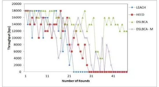
We compared classical clustering algorithms with the proposed algorithm in terms of packets sent, cluster count, energy and nodes alive. Simulation parameters are shown in Table 1. Each node assigns itself a random value between 0 and 1. If this value is less than the threshold, that node becomes a cluster head. Each node calculates its weight using equation (5) and (6), if the weight of any node is greater than the average weight of all the alive nodes then that node becomes the cluster head. DSLBCA and DSLBCA – M are compared with the classical algorithms such as LEACH and HEED. To compare the algorithms we used number of rounds referring the interval between initial clustering to clustering as well from one re-clustering process to another re-re-clustering process. Each round starts with a set-up-phase followed by steady-state-phase for forward the data to Sink. Algorithm with lesser dead nodes is chosen as the better one.
Table 1. Simulation Parameters
Parameters Values
Initial Energy 1 J
Transmission energy 50 nJ
Reception energy 50 nJ
Free space energy (Efs) 10 pJ
Multipath fading energy (Emp) 0.0013 pJ
Data Aggregation Energy (EDA) 5 nJ
Area 10000* 10000 m2
Packet size: Join message (Pjm)
Acknowledgement (Pack)
Cluster head message (Pchm)
Packet size (Psize)
2000 Bits 2000 Bits 2000 Bits 2000 Bits
Coordinates of the Sink (50,175)
Number of nodes 1000
Number of rounds 100
[image:5.595.162.435.277.426.2]Speed of the Mobile node (Mobile Environment) 0.02 m/sec
Figure 1. Throughput of the network for various algorithms
The number of clusters formed per round in both the algorithms is initially the same as shown in Figure 2. But with rounds it can be seen that there are more clusters in the case of DSLBCA as compared to LEACH, HEED and DSLBCA - M. The number of clusters to be formed assigned as 10 and over the iterations it is identified that after 25% of iterations (25 rounds) only less number of nodes in the LEACH are alive and they form as a single cluster. The performance of HEED is good upto 35% of iterations and due to stable clusters in DSLBCA shows less number of clusters and is maintained constant over iterations compared to the mobile DSLBCA (DSLBCA-M), in the later stages shows due to mobility factor DSLBCA-M frequently changes topology and a prey to frequent re-clustering.
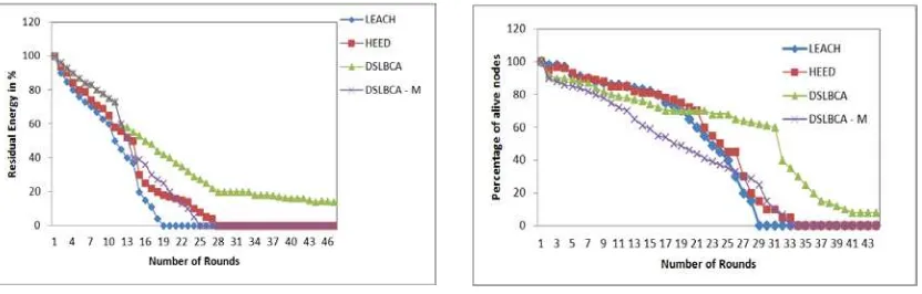
To analyse the energy efficiency node number 70 is chosen to compare its energy consumption subject to various algorithms. Figure 3 shows the residual energy level in the algorithms is initially same. At 30% and 50% of rounds it can be seen that the residual energy in node 70 is more in the case of DSLBCA about 11% and 13%, finally reaches 19% at the end of 100 rounds as compared to LEACH, HEED and DSLBCA - M.
Figure 2. Number of clusters of the network for various algorithms
Figure 3. Residual energy of the nodes for various algorithms
Figure 4. Alive nodes in the network for various algorithms
The proposed algorithms shown improved results by energy saving and dead nodes count over multiple rounds. Even after several iterations we are able to witness the performance of stationary nodes and fixed CH’s showing better results than the mobile nodes due to link stability and topology changes.
5. Conclusion
In this article, we proposed a distributed load balancing clustering algorithm for WSNs, considering optimal threshold for clusters configuration. Compared with LEACH, HEED and DSLBCA - M algorithm, the proposed algorithm supports to form a static cluster and improved network life time. The simulation result shows that the algorithm is more stable and improved performance about 15% overall considering residual energy and network life time. Considering the practical implications we have used 10000 x 10000 area with 1000 nodes to for our analysis and found that the proposed scheme is showing improved results for both static and mobile environment proving the scheme supporting scalability and supports network of different sizes. Hence in our future work we planned to focus on how to enhance this network through interfacing it with internet using real sensor nodes with industrial standards (Zigbee) for communication.
References
[1] Reen-Cheng Wang, Ruay-Shiung Chang, Jei-Hsiang Yen, Pu-I Lee. A Dynamic Topology Reformation Algorithm for Power Saving in ZigBee Sensor Networks. International Journal of
[image:6.595.94.510.292.425.2][2] Santar Pal Singh, SC Sharma. A Survey on Cluster Based Routing Protocols in Wireless Sensor
Networks. International Conference on Advanced Computing Technologies and Applications
(ICACTA). India, Mumbai. 2015; 45: 687-695.
[3] Xinfang Yan, Jiangtao Xi, Joe F Chicharo, Yanguang Yu. An Energy-Aware Multilevel Clustering
Algorithm for Wireless Sensor Networks. IEEE International Conference on Intelligent Sensors,
Sensor Networks and Information Processing. Sydney, Australia. 2008: 387-392.
[4] Julia Albath, Mayur Thakur, Sanjay Madria. Energy Constraint Clustering Algorithms for Wireless Sensor Networks. Ad Hoc Networks. 2013; 11(8): 2512-2525.
[5] Zhidan Liu, Wei Xing, Yongchao Wang, Dongming Lu. Hierarchical Spatial Clustering in Multihop Wireless Sensor Networks. International Journal of Distributed Sensor Networks. 2013; 11.
[6] Choon-Sung Nam, Young-Shin Han, Dong-Ryeol Shin. The Cluster-Heads Selection Method considering Energy Balancing for Wireless Sensor Networks. International Journal of Distributed
Sensor Networks. 2013; 6.
[7] Wendi B Heinzelman, Anantha P Chandrakasan, Hari Balakrishnan. An Application-Specific Protocol Architecture for Wireless Microsensor Networks. IEEE Transactions on Wireless Communications.
2002; 1(4): 660-670.
[8] A Muthulakshmi, S Hariraman. Load Balanced With Distributed Self Organization in File Sharing and File Accessing. International Journal on Recent and Innovation Trends in Computing and
Communication. 2014; 2(5); 990-996.
[9] V Windha Mahyastuty, A Adya Pramudita. Low Energy Adaptive Clustering Hierarchy Routing Protocol for Wireless Sensor Network. TELKOMNIKA. 2014; 12(4): 963-968.
[10] Y Liao, H Qi, W Li. Load-balanced clustering algorithm with distributed self-organization for wireless sensor networks. IEEE Sensors Journal. 2013; 13(5): 1498-1506.
[11] Khalid Haseeb, Kamalrulnizam Abu Bakar, Abdul Hanan Abdulla, Adnan Ahmed. Grid Based Cluster Head Selection Mechanism for Wireless Sensor Network. TELKOMNIKA. 2015; 13(1): 269-276. [12] M Chatterjee, SK Das, D Turgut. WCA: A weighted clustering algorithms for mobile ad hoc networks.
Cluster Computing. 2002; 5(2): 193-204.
[13] Y Fernandess, D Malkhi. K-clustering in wireless ad-hoc networks. Proceedings of the second ACM international workshop on Principles of mobile computing. 2002: 31-37.
[14] M Lehsaini, H Guyennet, M Feham. A novel cluster-based selforganization algorithm for wireless
sensor networks. International Symposium on Collaborative Technologies and Systems, 2008. CTS
2008.Irvine, USA. 2008: 19-26.
[15] N Mitton, B Sericola, S Tixeuil, E Fleury, IG Lassous. Self-stabilization in Self-organized Wireless Multihop Networks?. Ad Hoc & Sensor Wireless Networks. 2011; 11(1-2): 1-34.
[16] Zhenquan Qin, Can Ma, Lei Wang, Jiaqi Xu, Bingxian. An Overlapping Clustering Approach for Routing in Wireless Sensor Networks. International Journal of Distributed Sensor Networks. 2013; 11. [17] Hooman Hematkhah, Yousef S Kavian. DCPVP: Distributed clustering protocol using voting and
priority for wireless sensor networks. Sensors (Switzerland). 2015; 15(3): 5763-5782.
[18] Jie Wu, Liyi Zhang, Yu Bai, Yunshan Sun. Cluster-based consensus time synchronization for wireless sensor networks. IEEE Sensors Journal. 2015; 15(3): 1404-1413.
[19] B Baranidharan, S Srividhya, B Santhi. Energy efficient hierarchical unequal clustering in wireless sensor networks. Indian Journal of Science and Technology. 2014; 7(3): 301-305.
[20] Ying Liao, Jianjing Shen, Yi Lin, Changlin Zhou. Quantitative analysis of network configuration in randomized distribution wireless sensor networks. IEEE Sensors Journal. 2014; 14(6): 1974-1979. [21] Upasana Dohare, DK Lobiyal, Sushil Kumar. Energy balanced model for lifetime maximization in
randomly distributed wireless sensor networks. Wireless Personal Communications. 2014; 78(1): 407-428.