Conditional Residual Time Modelling Using Oil Analysis: A Mixed Condition Information Using Accumulated Metal Concentration and Lubricant Measurements.

(1)

IMEC2006, ChengDu, China A-1

Proceedings of ICME2006: International Conference on Maintenance Engineering ChengDu, China October 15-18, 2006

Conditional Residual Time Modelling Using Oil Analysis: A Mixed Condition Information Using Accumulated Metal Concentration and Lubricant

Measurements

Burairah Hussin and Dr. Wenbin Wang Centre for OR and Applied Statistics University of Salford, Salford M5 4WT, UK

This paper reports on modelling decision problems associated with condition monitoring by providing some scientific support to maintenance decision making. In this study, a Spectrometric Oil Analysis Programme (SOAP) is used as monitoring measures for diesel engines used in ships. Using the residual time at a monitoring check as the condition of the diesel engines, we seek to establish the relationship between the residual time and the total wear concentrations which are available from SOAP data. These metal concentrations are treated as concomittent variables which are influenced by the residual time. We also used lubricant measurements data acting as covariates that may increase/decrease the residual time. The formula for finding a residual time distribution is presented using a filtering technique and a method for estimating the model parameters is discussed. Once the distribution of the residual time is known, a decision model can be established to recommend the optimal maintenance actions in terms of cost, availability or any criterion of interest.

Key words: residual time, oil analysis, modelling decision problems, filtering technique

1. INTRODUCTION

(2)

In a parallel work, (Hussin and Wang, 2006) we had shown how the residual time of an engines used in ships can be modelled using total metal concentrations based on SOAP analysis. However, SOAP analysis can detect metals element up to 8 microns in size, which implied that the larger metals are not detected. Hence, we might not capture more information that could tell us about the exact accumulated metal concentration in engines. However, SOAP also provides lubricant performance measures as an indicator of lubricant performance, which could influence the engine wear. Hence, we are interested to develop a residual time prediction model that combined the information given by metal concentration and the lubricant data.

2. MODELLING DEVELOPMENT

This development of a new model is similar with a model which had developed in other works, (Wang and Christer, 2000; Wang, 2002; Wang, 2004), (Zhang, 2004) and (Wang and Zhang, 2005) but with a few new extensions as we embed lubricant data as a factor that could increase or decrease the residual time. For the purpose of model building, we list notation as follows:

2.1 Notations

i

x is a residual time at time t_i.

i

y is a type of concomittent monitoring information which reflects the condition of the engine state. y_i is random and the relationship between x_i and y_i is described as p(y_i |x_i).

i

z is a type of covariate monitoring information which may influence x_i but is assumed not having influence in y_i. This is because if both of the measurements are correlated, it is sufficient to use only one measurement. Thus, at this early stage, a simple analysis has been carried out from data that support our assumption, that there are no correlation between y_i and z_i.



i

x is the residual time before information z_i is taken at time t_i. In our case, both information

i

y and z_i are available at the same time. 

i

x is the residual life after the information z_i is taken at time t_i.

i

Y and Z_i are the monitoring history for y_i and z_i which takes the values of



y1,y2,,yi



, z1,z2,,zi



.

2.2 Formulations

Our objective is to find the residual time distribution given the information of metal

concentration and lubricant data, i.e. p(x_i |Y_i,Z_i) at time t_i. To start with, we defined the residual time adopted from (Wang and Christer, 2000) as

 

  

  



defined not

)

( 1

1 i i

i i

t t x x

otherwise ,

if x_i_₁ t_i t_i_₁ no maintenance intervention,

(1)

The relationship between x_iand x_i can be shown as below 

i

x = Bzi i e

x 

(2)

where B is a parameter that defines the influence of z_iand z_i is z_i z_i_₁. Noted that if

i

z

(3)

IMEC2006, ChengDu, China

where M is the size of the vector. For the sake of simplicity, we will use a scalar to explain the influence of z_i in the model. We will deal with this vector while fitting the model with data. Hence, equation (2) and (3) can be explained as follows,

1. if z_i 0, then x_i x_i which means the residual time remains the same.

2. if z_i 0, x_i x_i which means the residual time becomes shorter, the system is deteriorating.

3. if z_i 0, x_i x_i which means the residual life becomes more longer, the system is improving.

We seek to establish the p(x_i |Y_i,Z_i) and adopted from (Wang and Christer, 2000), it can be

and after some manipulation, equation (4) can be written as

)

Equations (4) and (5) are important that explained how the condition monitoring data is taking into account in the model with two key issues that need further explanation. x_i measures the residual time from new, taking consideration the concomittent variables and covariates. Since

0

Y and Z0, are not available at t0 in most cases, we therefore set p(x0 |Y0,Z0) p(x0)

 _,

which is the pdf of the machine life.

The next stage is to establish the relationship between the observed information, y_i and z_i,

with the residual time,x_i, which can be established by a probability distribution (Wang and

Christer, 2000). Generally, we expect that a short residual time, x_i, will generate a high reading in y_i. However, taking consideration of covariates, z_i should increase or decrease the

(4)

IMEC2006, ChengDu, China

3. PARAMETER ESTIMATION

To be able to use equation (6) we need to know the parameters within equation (6). The model parameters are estimated in two steps, with the first step is to estimate the parameters in p(x₀), namely , the scale, and , the shape parameters of the Weibull distribution as a failure distribution. This can be done because from our assumption that y_i is dependent on

i approach becomes,

)

(5)

In order to fit data to the model, we need to prepare data that is suitable for the model’s

requirements. To prepare the required data from metal element information, we used the analysis that yields total wear metal concentrations, (Hussin and Wang, 2006). For data preparation from oil performance measurements, instead of using the original oil data values, we applied a concept called independent component analysis (ICA). This is carried out for two main reasons; the first is to normalize the scale of each individual oil performance measurement and the second is to identify the possibility of reducing the dimensions of the monitored variables for oil performance. Normalization of the scale of the parameters is important, as each parameter has its own scale and it was noted from the literature, (Lukas and Anderson, 1996) and discussion with persons familiar with similar types of data that these variables are very much correlated among themselves. Therefore, ICA can be used to calculate the contribution of each parameter.

4.1 Independent Component Analysis (ICA)

ICA of a random vector X consists of finding a linear transformation sˆWx so that the components sˆ_i are as independent as possible, in the sense of maximizing some function

)

ˆ

,...,

ˆ

(s₁ s_m

F that measures independence. To begin the discussion of ICA, we can express the entire system of n measured signals and m observations as

As

x :

    

    

    

          

    

n mn m

n

m s

s

a a

x x

: : :

:

1

1 11

1

 

(9)

We refer to each original independent signal as s. Each measured signal x can be expressed as a linear combination of the original independent signals. A is an mn mixing matrix that generates x from s. Hence, the goal of ICA, given the observation x, is to calculate matrix A and the set of independent s values. In order to perform this task, our intention is to find a matrix W(the inverse ofA) such that, if it is applied to x, it yields a dataset sˆ that is as independent as possible and thus approaches the unknown signals s.

Wx sˆ :

    

    

    

          

    

m n m n

m

n x

x

w w

s s

: : :

ˆ

:

ˆ 1

1

1 11

1

 

(10)

(6)

further analysis. As noted above, ICA has the possibility of reducing the dimensions of the variables, although this is not it main purpose. This analysis was conducted on our data set, and while conducting the whitening process, the eigenvalues of the first principal component of uncorrelated variables showed a range of values from 55 to 95%. This strongly suggests that the dimensions could not be reduced, hence we decided to use the entire set of variables in the model. Having all the data required in hand, we first estimated the parameter values for our model. We randomly selected 22 sets of data for this purpose and the results are shown below.

Table 1: Estimated parameters from observed data

a b  B₁ B2 B3 B4

0.00106 0.00021 1.19712 0.03321 0.01672 0.03516 0.06309

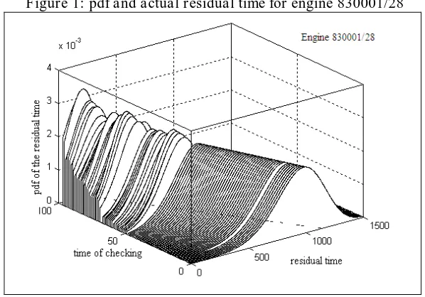
The variances of the estimated parameters are relatively small for all parameters, which tell us something about variability around the mean. Thus, we can say that the parameter estimates were good. The covariance of each parameter is literally small, indicating that there are no relationships between variables. Using the estimated parameters, we calculated our residual model, p(x_i |Y_i,Z_i), using the remaining dataset. Figure 1 below shows one of the results for residual time distribution. The dotted straight line in the plot indicates the actual residual life. It is shown that the variance of the pdf of the residual time becomes smaller as we have more information.

Figure 1: pdf and actual residual time for engine 830001/28

5. MODEL COMPARISON

(7)

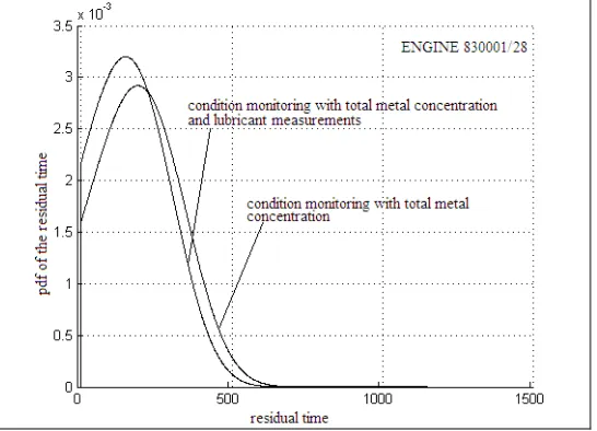
Figure 2: pdf residual time of engine 830001/28 at the last observation point using total metal concentration.

5.1 The Decision Model

The essential decision to make at different monitoring point is whether we should replace the engine or not given all information available. If the answer is yes then what is the best time for such replacement, and should we wait until a suitable production window such as a scheduled shutdown arrives? Suppose, we need to develop a decision model, therefore a

decision variables itself might depend on several criteria’s such as cost, reliability, safety or

any criterion of interest. To show an example, we adopt a decision model developed by (Wang and Christer, 2000) as





 

 

 

  

 



 T t

i i i

i i

i p i i

i f

dz Y z zp Y

t T x P t T t

Y t T x P C Y t T x P C t C

0

) | ( ))

| (

1 )( (

)) | (

1 ( ) | (

)

( ₍₁₁₎

where ) (t

C is the total expected cost per unit time

t is the current monitoring point measured from new T is the planned replacement time

) |

( _i _i

i x T t Y

P   is the probability of the residual time at time t

f

C is a failure cost

p

C is a preventive cost

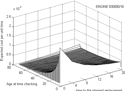
The decision model above assumes that the cost monitoring cost is negligible. Suppose that the mean cost of a failure replacement is 10 times higher than the mean cost for a preventive maintenance, using the estimated parameter and equation (11) above we compute the decision model on a life dataset. At every at every t time, we could identify the best time to carry out a preventive replacement, T. We show one example. The diesel engine is monitor for 72 data points from new and the interval between monitoring is 9.2 days and failed at 658.2 days of operation. We notice that from

Figure 3 that the expected cost per day is decreasing at early stage until it starts to increase at th

(8)

Figure 3: Expected cost per day in terms of planned replacement at time t given that the current monitoring check is time t

6. CONCLUSION

This paper has outlined a new development of conditional residual time where the previous approach is enhanced with some data that we assume will increase or decrease the residual time. This was done by first assuming that the residual time is a function of observed concomittent monitoring data, y. Then, we set up a relationship indicating how the residual time will change with the covariates, z. Issues such as the possibility of the covariates being correlated with each other were solved by using ICA. By providing the data required by the model, we then estimated the model parameters using the maximum likelihood approach. The results from parameter estimation were sufficiently good to justify proceeding with fitting the model to the data. The results of this approach were satisfactory, showing better prediction than the previous model with the same dataset. Thus it is concluded that more information leads to better a prediction.

REFERENCES

Hussin, B. and W. Wang (2006). Maintenance Decision Making Using Condition Monitoring Data: A Study From Oil Analysis Salford Postgraduate Annual Research Conference, Salford, University of Salford.

Hyvärinen, A. and E. Oja (1997). "A Fast Fixed-Point Algorithm for Independent Component Analysis. , 9, 1483-1492. ." Neural Computation(9): 1483-1492.

Lukas, M. and D. P. Anderson (1996). "Lubricant Analysis for Gas Turbine Condition Monitoring." American Society of Mechanical Engineers(Paper): 1-12.

Wang, W. (2002). "A Model to Predict the Residual Life of Rolling Element Bearings Given Monitored Condition Information To Date." IMA Journal of Management

Mathematics 13: 3-16.

Wang, W. (2004). Modelling identification of the initial point of a random fault using available condition monitoring information. 5th IMA International Conference, University of Salford, UK.

Wang, W. and A. H. Christer (2000). "Towards A General Condition-based Maintenance Model For A Stochastic Dynamic System." Journal of The Operational Research Society 51(2): 145-155.

(9)