Selecting a linear mixed model for longi

0F1F2F3F4F5FRunning head: SELECTING A LINEAR MIXED MODEL

Selecting a linear mixed model for longitudinal data: Repeated measures

ANOVA, covariance pattern model, and growth curve approaches

Siwei Liu

Michael J. Rovine

Peter C. M. Molenaar

The Pennsylvania State University

Author Note

Siwei Liu, Human Development and Family Studies, The Pennsylvania State

University; Michael J. Rovine, Human Development and Family Studies, The Pennsylvania

State University; Peter C. M. Molenaar, Human Development and Family Studies, The

Pennsylvania State University.

This study was supported by a grant from the National Science Foundation (NSF

0527449) to the second author. These data have not been published anywhere and have not

been submitted for publication anywhere else.

Correspondence should be addressed to Siwei Liu, Human Development and Family

Studies, 110 S-Henderson, The Pennsylvania State University, University Park, PA 16802.

Abstract

With increasing popularity, growth curve modeling is more and more often considered as the

first choice for analyzing longitudinal data. While the growth curve approach is often a

good choice, other modeling strategies may more directly answer questions of interest. It is

common to see researchers fit growth curve models without considering alterative modeling

strategies. In this paper we compare three approaches for analyzing longitudinal data:

repeated measures ANOVA, covariance pattern models, and growth curve models. As all

are members of the general linear mixed model family, they represent somewhat different

assumptions about the way individuals change. These assumptions result in different

patterns of covariation among the residuals around the fixed effects. In this paper we first

indicate the kinds of data that are appropriately modeled by each, and use real data examples

to demonstrate possible problems associated with the blanket selection of the growth curve

model. We then present a simulation that indicates the utility of AIC and BIC in the

selection of a proper residual covariance structure. The results cast doubt on the popular

practice of automatically using growth curve modeling for longitudinal data without

comparing the fit of different models. Finally, we provide some practical advice for

assessing mean changes in the presence of correlated data.

Selecting a linear mixed model for longitudinal data: Repeated measures ANOVA, covariance pattern model, and growth curve approaches

Introduction

Developmental researchers often conduct longitudinal studies to examine stability and

change, in which individuals are measured on multiple occasions. Repeated measures of

individuals create challenges for data analysis because they are not independent. A variety

of models have been developed for analyzing longitudinal data (Hedeker & Gibbsons, 2006;

McArdle, 2009; Singer & Willett, 2003). However, it is often not clear to substantive

researchers which model to use or how to choose among different models. This confusion

sometimes leads to a naïve approach of fitting one particular model without consideration of

other alternatives. In particular, when the research question involves the assessment of

change over time, fitting a growth curve model seems to have become the standard in

developmental research. While the growth curve approach is often a good choice, other

modeling strategies may more directly answer questions of interest. In this paper, we argue

for a model-based selection procedure to determine the proper model for assessing mean

changes in the presence of correlated data. We use the linear mixed model (Laird & Ware,

1982) as a general framework and concentrate on three models that are subsumed under the

mixed model family: repeated measures analysis of variance (ANOVA; G. E. P. Box, 1954;

Myers, 1979; Scheffe, 1959), covariance pattern model (Hedeker & Gibbons, 2006), and the

multilevel growth curve model (Bryk & Raudenbush, 1992; Goldstein, 1995).

Before going into the details of the three models, it is necessary to clarify the scope of

Here, we focus on the most basic question in developmental research: how to model change

over time. When the data are assumed to come from a multivariate normal distribution, the

consideration of proper analytic strategy to answer this question consists of two parts: the

modeling of the means and the modeling of the residuals around the means. In the linear

mixed model framework, the means are modeled by fixed effects, which are identical for all individuals, whereas the residuals are modeled by random effects, which vary by individuals. Typically, we are primarily interested in estimating and testing hypotheses about the fixed

effects, and the covariance matrix of the random effects is of secondary interest. Repeated

measures ANOVA, covariance pattern model, and the multilevel growth curve model

represent different ways to model the fixed and random effects. Both repeated measures

ANOVA and the covariance pattern model treat time as a categorical variable and have a

saturated means model, thus, the means are modeled perfectly. They account for the

correlation of the residuals around the fixed effects model by allowing the covariance matrix

of residuals to show a particular pattern: compound symmetry or the less restrictive sphericity

for repeated measures ANOVA; one of a number of alternative patterns (e.g., autoregressive)

for the covariance pattern model. The multilevel growth curve model treats time as a

continuous predictor and assumes that the means across time follow a particular shape.

Individuals are assumed to follow the same curve shape but are allowed to vary in the

parameters that describe this curve (random effects). Variability in these parameters and the

individual deviations around this curve result in a residual covariance pattern different from

the ANOVA or covariance pattern models.

researchers, in this paper we focus on the selection of an appropriate model to account for the

correlations of the residuals around the fixed effects model. We use the term error structure

to refer to the covariance pattern of these residuals. For repeated measures ANOVA and the

covariance pattern model, error structure simply refers to the covariance pattern of errors.

For the growth curve model, it refers to the covariance pattern resulted from combining the

random effects and the errors around individual curves. The error structure is important

because it is included as a probability model in the maximum (or restricted maximum)

likelihood estimation of parameters. Identifying the best fitting error structure is often

recommended to obtain a proper inference related to tests of the fixed effects (Jennrich &

Schluchter, 1986; Milliken & Johnson, 2009). Since the “true” error structure is usually

unknown, some goodness-of-fit criterion is necessary to select the best error structure

(Jennrich & Schluchter, 1986). In the mixed model approach, we can use AIC (Akaike

information criterion; Akaike, 1974) and BIC (Bayesian information criterion; McQuarrie &

Tsai, 1998; Schwarz, 1978) to assess the goodness-of-fit.

With the increasing popularity of growth curve modeling, it is common to assume a

simple shape (e.g. linear) to the means. This assumption also implies a specific error

structure. Even if the means fall on a straight line, however, some other error structures may

represent a better fit to the data. This is often not tested.

In the following, we will first describe the presumed error structures of the repeated

measures ANOVA model, the covariance pattern model, and the growth curve model. Next,

we will apply these models to both real and simulated data to highlight the problems for

AIC and BIC to choose among different error structures when working with real data.

In this paper we will concentrate on complete data examples. Linear mixed models

programs such as SAS PROC MIXED handle missing data in the dependent variables

through the use of full-information maximum likelihood estimation (FIML) based on the raw

data likelihood (Littell, Milliken, Stroup, Wolfinger, & Schabenberger, 2006). More general

approaches such as multiple imputation (Schafer, 1997) can be implemented. Linear mixed

models are well suited to unbalanced designs (i.e., each individual is observed at potentially

different time points). For models discussed here, solutions for a number of unbalanced

designs are described in Milliken and Johnson (2009).

The General Linear Model (GLM) and the Linear Mixed Model (LMM)

Most researchers are familiar with the general linear model (GLM), which is usually

used to represent regression models. If y is an n×1 vector of scores on the dependent variable, and X is an n×kdesign matrix with one column representing a constant and k-1

columns representing the k-1 independent variables, then the general linear model of regression is:

ε

Xβ

y= + (1)

where ß is a k×1 vector of regression coefficients, and ε is an n×1 vector of errors with a distribution of N (0, σ_ε2I). The design matrix can include dummy coded variables to

represent groups, which then turn the model into an ANOVA model. The regression

estimator is:

) ( )

(XTX 1 XTY

β ₌ −

(2)

For the simple regression equation,

i i 1 0

i β β x ε

y = + + (3)

=

(

y

|

x

_i

)

+

ε

_i,

the observed value of the dependent variable, yi, is equal to the conditional mean of y given the value of xi plus the individual’s residual. Under the independence assumptions we estimate the values of the regression weights and the variance of the errors, . Under

normal theory these estimates can be used to provide a proper inference. When the

independence assumptions are violated, the inference becomes biased. The linear mixed

model produces a proper inference by allowing residuals to be correlated.

The linear mixed model (LMM) proposed by Laird and Ware (1982) based on the

work of Harville (1977) is expressed as:

i i i i

i X β Z γ ε

y = + + (4)

where the subscript i represents an individual or other unit of analysis (e.g. family) on which observations are repeated. yi is an ni×1 vector of response values for the ith individual, Xi is

an ni×b design matrix of independent variable values, ß is the corresponding b×1 vector of fixed effect parameters, Zi is an ni×g design matrix for the random effects, and γi is a g×1

vector of random effect scores. The fixed effects coefficients ß = (ß1, ..., ßb)T are common

among all individuals. The random effects γi= (γi1, ..., γig)T can vary by individual. They

are assumed to be normally distributed with means zero and a covariance matrix G. The εi

are within subject errors that are assumed to be normally distributed with means zero and a

covariance matrix σ_ε2Wi. While the number of observations and design matrix vector values

is measured on the same occasions (Xi=X; Zi=Z; Wi=W).

We can break down Equation 4 into a conditional means model and now a covariance

structure for the residuals where

β

X ) X | y (

yi = i i = i



is the fixed effects means model and

i i iγ ε

Z +

is the random effects model. The covariance matrix of the random components Ziγi + εi (i.e.,

the error structure) is given by:

W ZGZ

V= T +σ2_ε . (5)

This form is very general. We can model it using only the errors, εi. In this case, Z and G

would both be zero and we specify a pattern for σ_ε2W in terms of a set of variance and/or

covariance parameters - this is done in repeated measures ANOVA and the covariance pattern

model. As part of the estimation process we estimate the values of those parameters.

Alternatively, it may be more convenient to allow random regression weights for modeling

the residuals. This especially holds true in the case of growth curve modeling, where the

residuals can be modeled by an individual curve that deviates from the group curve and a set

of individual errors that deviate from the individual curve.

Once V is specified the Henderson (1990) mixed model estimator for the regression

weights is:

Y) V (X X) V (X

β = T −1 −1 T −1

. (6)

In contrast to GLM, the regression coefficients in LMM are dependent on the covariance

estimates (along with different standard errors). For that reason, it is especially important to

determine the best error structure when modeling any data set.

The Repeated Measures ANOVA Model

The repeated measures ANOVA model was first developed by Fisher (Scheffe, 1959)

to model mean differences based on an experimental design. In the original formulation, the

repeated measures factor represented a randomized ordering of a repeatedly administered

treatment factor.

A one-way repeated measures ANOVA can be presented as a LMM where Ziγi is zero:

i i Xβ ε

y = + (7)

(Rovine & Molenaar, 2000). For example, for a repeated measures design with 5 occasions,

the model can be written as:



where yi1 to yi5 are the individual’s scores at the 5 occasions. The fixed-effects coefficients

ß1, ß2, ß3, ß4, and ß5 yield the expected values for yi5, yi1 - yi5, yi2 - yi5, yi3 - yi5, yi4 - yi5,

respectively. The within-person residuals εi form a 5×5 covariance matrix, σε2Wi, which is

The covariance between occasions is assumed to be σ regardless of the distance between

occasions and the variance at each occasion is assumed to be σε2+σ. We estimate σand σε2

along with the fixed effects parameters.

The Covariance Pattern Model

The covariance pattern model (Hedeker & Gibbons, 2006; Jennrich & Schlucter, 1986;

Laird & Ware, 1982) can be thought of as an extension of the repeated measures ANOVA.

Its primary purpose is identical, namely, to model mean differences as expressed in the

conditional means model; but this model allows structures other than compound symmetry to

describe the error structure.

Jennrich and Schluchter (1986) introduced methods for modeling alternative error

structures related to their work on the development of a general procedure for implementing

the Laird-Ware mixed model (SAS PROC MIXED). Currently, SAS PROC MIXED

includes roughly 36 alternative structures. This greatly enhances the ability to model mean

differences, especially in the case of longitudinal data, where time, not treatment, is the repeated measures factor. To describe some of the options of the covariance pattern model,

we will concentrate on two patterns that represent qualitatively different structures than the

compound symmetry pattern described above: the first-order autoregressive (AR(1)) pattern, and the first-order moving average (MA(1)) pattern. Rovine and Molenaar (2005) have shown that based on the addition rules of Granger and Morris (1976), any other covariance

pattern can be constructed as a sum of autoregressive and moving average components.

residual correlations. One pattern that allows this structure is the first-order autoregressive

or AR(1) structure. For 5 occasions of measurement this structure is:

σε2

results from the first-order autoregressive process:

it 1) i(t it ρε υ

ε = ₋ + (9)

where the innovation υit is normally distributed with mean zero. It assumes that the

correlation of errors between any two consecutive occasions is identical; thus, the correlation

decreases at a constant rate as two measurements get farther away in time. This structure

differs from compound symmetry which assumes that the covariance of residuals between

any two occasions is identical. For longitudinal data it may be unreasonable to assume that

the residual covariance between distant occasions is the same as the covariance between

adjacent occasions.

The MA(1) pattern. When a process cuts off after a certain number of occasions, a good model for that structure is the moving average pattern. The first-order moving

average (MA(1)) pattern is:

σε2

between more distant occasions is zero. As we can see, the larger the value of γ, the more

this diverges from compound symmetry.

Unlike ordinary regression, the covariance of the residuals is part of the linear mixed

model estimator. As a result, the fixed effects estimates, β, are affected by the presumed

error structure. The probability of jointly observing the data depends on properly modeling

the fixed effects and properly describing the distribution of the errors.

The Multilevel Growth Curve Model

The multilevel growth curve model combines two complementary traditions: growth

models first described independently by Tucker (1958) and Rao (1958), and linear mixed

models described by Henderson (1953) and Hartley and Rao (1967). Equivalent statistical

methods for analyzing multilevel data have been developed and described. Here, we

concentrate on two methods: the linear mixed model approach (Laird & Ware, 1982; Littell et

al., 2006; Rosenberg, 1973), and the multilevel approach (Bryk & Raudenbush, 1992;

Goldstein, 1995). Growth curve models can also be implemented as structural equation

models (SEM; Bauer, 2003; Curran & Bauer, 2007; Rovine & Molenaar, 2000). Alternative

estimation approaches for these methods include empirical Bayes estimation (Bryk &

Raudenbush, 1992) and the estimator resulting from the Henderson mixed model equations

(Henderson, 1990). Estimators from these two general methods have been shown to be

equivalent (Littell et al., 2006; Robinson, 1991).

In the form of a multilevel model, a simple linear growth curve model is:

where π0i and π1i are individual intercepts and slopes, εit are errors around individual lines that

are typically assumed to be independent and normally distributed with constant variances

over time (although this assumption can be relaxed in SEM), ß00 and ß10 are the average

intercept and slope, υ0i are differences between the individual and average intercepts, and υ1i

are differences between the individual and average slopes. We can transform this into the

linear mixed model form by combining the level 1 and level 2 equations. We then get:

it

The error structure for this model is based on having a set of random effects that reflect the

fixed effects model. More generally, methods for properly selecting the set of random

effects to include in growth curve models have been described (Gelman & Hill, 2007;

Maxwell & Delaney, 2004).

Suppose the data comes from a repeated measures design with 5 equally spaced

occasions, a linear growth curve model with random intercept and slope can be written as:

and σis is the covariance between the random intercepts and slopes. The error structure of

the this model can be called the random-coefficients (RC) structure (Wolfinger, 1996). As demonstrated by Rovine and Molenaar (1998) and Biesanz, Deeb-Sossa,

Papadakis, Bollen, and Curran (2004), the magnitude of σis, the covariance between random

intercepts and slopes, depends on the placement of the intercept, which is often an arbitrary

decision made by researchers. For simplicity, we show here the random-coefficients

structure for a five-occasion linear growth model with σis=0:



This pattern assumes a functional relationship among variances along the diagonal over time

and a functional relationship among covariances over time which depends on the spacing

between occasions1. In the case that all individual trajectories are parallel to the group

trajectory, the terms related to σs2 are all 0 and the pattern reduces to compound symmetry.

With small variation in the individual slopes, the linear growth curve error structure and

compound symmetry are almost indistinguishable. As the variability in the slopes increases,

the two patterns diverge.

Writing the Repeated Measures ANOVA and Covariance Pattern Models as a Multilevel

Model

To help compare the repeated measures ANOVA and the covariance pattern model to

1

The pattern showed here results from the specific way in which we specified the random effects. In general,

the growth curve model, we can alternatively express them as multilevel models. With five

repeated occasions they become:

Level 1: y_it =π_0i+π_1iυ₁+π_2iυ₂+π_3iυ₃+π_4iυ₄+ε_it (13)

effects at level-2. This is because the covariance structure is completely modeled by

patterning the level-1 εits. If we choose compound symmetry, we have the standard repeated

measures ANOVA. By selecting another structure, we would have a covariance pattern

model.

An alternative way to model the compound symmetry structure would be to include a

random intercept only along with a diagonal covariance matrix of the εit. For this model the

first equation of level-2 becomes:

i

Everything else remains the same. This alternative would be analogous to a growth curve

model in which all of the individual curves are parallel differing only in level, not in slope.

In this case, all of the occasion residual variances would be modeled as identical and the

residual covariances would all be the same.

A comparison among repeated measures ANOVA, the covariance pattern model, and

the growth curve model shows two of the modeling decisions that the researcher must make.

First, what is the proper fixed effects model for the data? When the fixed effects

model cannot be hypothesized a priori, it must be determined empirically. One of the decisions we have to make when modeling the means is whether to treat time as categorical

or continuous. In repeated measures ANOVA and the covariance pattern model, time is

discrete and treated as a categorical variable, whereas in the growth curve model, time is

continuous. Hence, growth curve models are more convenient when dealing with data

where individuals are measured at varying occasions (unbalanced design). In many

developmental studies, researchers are only interested in changes in a construct across several

time points, and each participant is measured on the same occasions (balanced design). In

this case, treating time as a categorical variable may be more appropriate. When we have a priori hypotheses about the means, such as a straight line, a linear growth curve model can be fitted. Alternatively, in ANOVA or the covariance pattern model, we can use a linear

polynomial as a planned contrast “predictor variable”. The variability around this straight

line could then be modeled using, for example, a compound symmetry error pattern.

Second, what type of error structure best fits the data? When certain parameter

values are small, the difference between structures can be indistinguishable. When the

variability in the random slopes is small, the random-coefficients structure assumed by the

linear growth curve model is very similar to compound symmetry. When the correlation

between adjacent occasions is very small, compound symmetry, AR(1), and MA(1) may be

approaches zero, AR(1) and MA(1) may be indistinguishable. However, using different

structures in the model estimation may lead to differences in the inferences. Even when

different error structures all lead to significant results, they can have different effect sizes

which can change the interpretation of the results.

With the increasing popularity of growth curve modeling, the above decision making

process is often ignored. In particular, the linear growth curve seems to be the model of

choice these days. With the linear growth curve model as the only model considered,

researchers fail to consider 1) whether the data follow the pattern assumed by the model (i.e.,

do all individuals follow a straight line?), and 2) whether an alternative model may better fit

the data. In the following, we use two real data examples to illustrate the potential problems

with this approach.

Two Real Data Examples

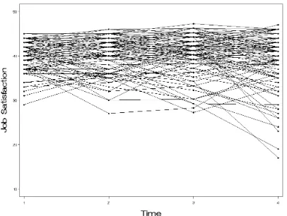
As part of a study by Belsky and Rovine (1990) a measure of job satisfaction was

collected on four occasions for husbands from families expecting a child. The data were

collected at roughly 3-month intervals with the first occasion occurring about 3 months

before the baby was due. A plot of the means along with fitted intercept and slope model

appears in Figure 1a and shows a generally decreasing mean pattern2.

[FIGURE 1A ABOUT HERE]

We first analyzed the data using a straight line growth curve model. The estimated

2

The original data had a quadratic trend (Belsky & Rovine, 1990). To concentrate on the linear growth curve,

we rescaled the data by shifting the third data point by a constant for all individuals. After rescaling, there was no significant higher order polynomial trend in the data and the original covariance structure of the residuals remained unchanged. The original data also showed idiosyncratic patterns and the growth curve error structure

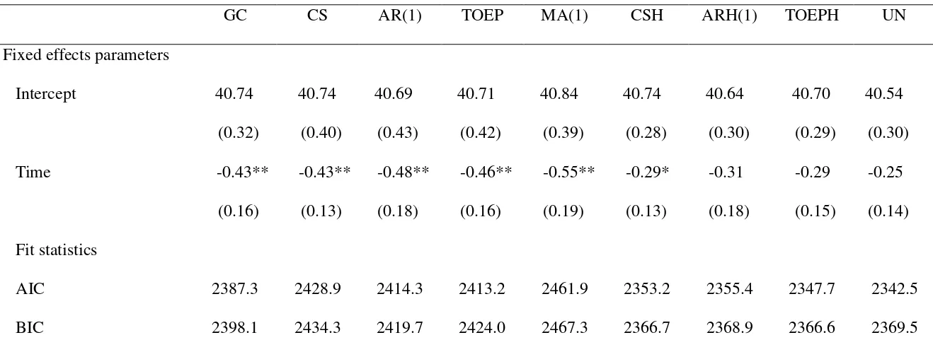
intercept and slope along with the standard errors appear in Table 1. To assess the relative

fit of the model, we included AIC and BIC. A smaller number in AIC and BIC indicates a

better fit (more details about AIC and BIC are given in the methods section). We next

analyzed the data using a straight line fixed effects model with some alternative error

structures that have been shown to represent plausible structures for longitudinal data3.

Looking at the table we see that the best fitting error structure according to AIC was

UNSTRUCTURED (UN) and according to BIC was TOEPLIZ with HETEROGENEOUS

variances (TOEPH). According to these models, the time effect is not significant, whereas

according to the standard growth curve model it is significant. If we assume for now that

the best fitting model according to AIC and BIC is closer to the “truth” (which will be tested

in the simulation study described later), the standard growth curve model is likely to have

resulted in a Type I error.

[TABLE 1 ABOUT HERE]

This result indicates that when individuals do not follow a common trajectory, the

standard growth curve model may not be appropriate. We can see evidence of these

different trajectory shapes by looking at a spaghetti plot of the observed data (Figure 1b),

3

No golden rule exists for determining the number and type of error structures to include in the comparison when dealing with real data. The error structures we included in this example are typical of those one might

see in longitudinal studies. CS is the structure assumed under traditional analysis of variance and often represents the structure when the repeated measures effect is a randomized ordering. AR(1) is often appropriate when more adjacent errors are more correlated than more separated errors. Toeplitz is a

generalized autoregressive model and allows errors at different spacings to have different correlations. MA(1) indicates a process in which the adjacent errors are correlated, but more distal errors are uncorrelated. Since the homogeneity of error variances across occasions may not hold, we also included heterogeneous versions of

these structures. Researchers should feel free to include additional structures or test fewer structures if they have a good reason of doing so. One could, for example, begin with an unstructured covariance pattern as a

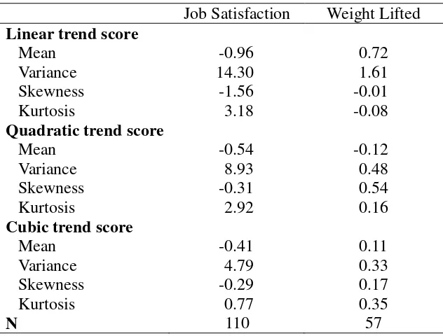
which seems to indicate that no typical trajectory exists for these individuals. We can also

see this by calculating a set of orthonormalized polynomial trend scores. Looking at the

variances (Table 2), we see that the individual linear trend had a relatively large variance and

somewhat less but still sizable variances for the individual quadratic and cubic trends. This

suggests idiosyncratic change rather than a common trajectory shape. For this scenario, the

growth curve error structure which is based on a common trajectory shape for each individual

may improperly account for the true covariance structure of the residuals.

[FIGURE 1B AND TABLE 2 ABOUT HERE]

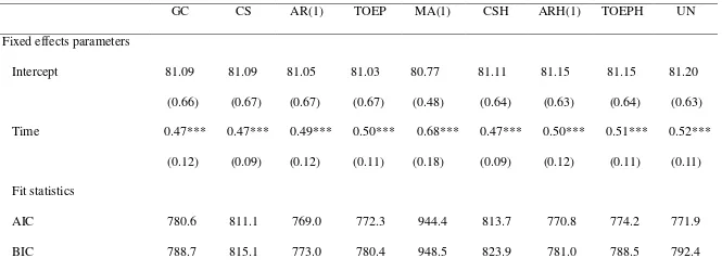
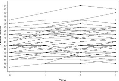
Littell et al. (2006) presented data from a study of strength resulting from different

programs of weight training. In this study, the amount of weight lifted was measured on a

number of occasions. We look at the first four occasions. From the spaghetti plot (Figure

2) and the distributions of the orthonormalized polynomial components (last column in Table

2), we see that unlike the previous example, the variances of the quadratic and cubic trends

are very small. The predominant individual trajectory is a straight line. Given this we may

expect the standard growth curve model to have a good fit to the data. However, the

variances of the errors around the fixed effect straight line regression model do not follow the

strict functional relationship we would expect under this model. Testing a number of

different error structures, we see that the AR(1) error structure around the straight line means

model is optimal for these data (Table 3). Comparing the results of the standard growth

curve model to AR(1), we see that although both models give significant results, the estimates

are different. In this case, the standard growth curve model underestimated the time effect.

random-coefficients error structure assumed by the linear growth curve model may still not

be optimal.

[FIGURE 2 AND TABLE 3 ABOUT HERE]

Other examples could be selected to show that the linear growth curve model can be

the preferred model over the others tested. We present these counter examples primarily to

indicate that the blanket selection of the growth curve model may result in a less than optimal

inference. Hence, selecting an error structure is an important part of the inferential process.

Given that, we next consider how feasible it is to select the “correct” error structure. We can

only demonstrate when we know what the true error model is, so we will investigate whether

our model comparison approach can recover the true model. This is an important

consideration in evaluating any statistical technique, because if the method cannot select the

correct model when the true model is known, we have less confidence in its ability to select

among a set of competing models. Conversely, if the method can select the true model

under a variety of conditions, we have more confidence in its general utility for selecting a

best model.

To investigate the degree to which comparative fit criteria can select a model when

the “true” model is known, we simulated data which have a straight line means pattern and

one of four error structures: compound symmetry (CS), AR(1), MA(1), and

random-coefficients (RC). These error structures represent, in order, the repeated-measures

ANOVA model, two covariance pattern models, and the linear growth curve model with

random intercept and slope, and are typically thought to represent qualitatively different

exhaustive set, we feel that these four patterns are different enough to allow us in this initial

investigation to examine whether AIC and BIC are able to identify the correct error structure

under various conditions.

Since AIC and BIC will not always select the proper model, we examine the degree to

which the inference of the time effect is affected. We discuss the extent to which our results

can be generalized to guide real data analysis in the discussion section.

Method Simulation

We simulated data based on a linear means model4. Specifically, all data were

assumed to come from a repeated measures study with five equally spaced occasions. The

means from the first to the last occasions were set to 5, 10, 15, 20, and 25, respectively. The

covariance matrix of residuals was simulated to show one of the following patterns.

Compound symmetry. A covariance matrix showing the compound symmetry

pattern was shown on page 9. To simulate data with this error structure, we used a

three-factorial design. The first factor was effect size, which contained two levels: medium

(.5) and large (.8) (Cohen, 1988). The second factor was intraclass correlation (ICC), which

had three levels: small (ρ=.2), medium (ρ=.5), and large (ρ=.8). Finally, we also varied the

sample size to be small (20), medium (100), or large (200). We chose these numbers

because they were representative of the spectrum of values in typical developmental research.

To construct the covariance matrix, we used the formula:

4

d = ' M -M_{1 2}

σ (14)

(Cohen, 1988) where d is the effect size, M1-M2 is the difference between two means, and σ'

is the standard deviation. In our simulation, M1-M2 was the mean difference between two

adjacent time points, and σ' equaled to the square root of the elements on the main diagonal

of the covariance matrix. Hence for a compound symmetry structure,

σ' = σ_ε2 +σ (15)

Combining the formula for intraclass correlation:

ICC =

σ σ

σ

ε2 +

(16)

we solved for σε2 and σ. All together, the three-factorial design yielded 18 (2×3×3)

combinations of simulation values. These values were in line with other similar studies

(Ferron, Dailey, & Yi, 2002; Keselman, Algina, Kowalchuk, & Wolfinger, 1999; Kwok, West,

& Green, 2007).

AR(1). To simulate data with an AR(1) structure (page 11), we again used a

three-factorial design, with the same values for effect size and sample size. Intraclass

correlation was replaced by the autoregressive coefficient, ρ, which again could vary from

small (0.2), medium (0.5) to large (0.8). Therefore, our simulation yielded 18 combinations

of simulation values for the AR(1) structure.

MA(1). The MA(1) pattern was shown on page 11. We used the same

three-factorial design, where the factors were effect size, sample size, and the moving

average coefficient, γ. Because γ has to be less than or equal to 0.5 for the covariance

combinations of simulation values.

Random-coefficients structure (RC). Because Z was constant, the RC structure

was determined by σ_ε2 and G = _

. To make the RC covariance matrix comparable

to the other structures, we set the value of σ_ε2 and σi2 as equivalent to the σε2 and σ in

compound symmetry. That is, the variance at the first occasion in RC was the same as the

variance in the CS, AR(1), and MA(1) structures. Moreover, we defined a ratio:

r =

which could be either small (0.1) or medium (0.25). This parameter controlled the rate of

change in variance and covariances over time. Because σis is arbitrary and subject to scaling,

it was set to 0. The simulation of the RC structure thus followed a four-factorial design,

with r as the added factor. We used a medium effect size (0.5), and small (20) and medium (100) sample sizes. In total, there were 12 (1×2×3×2) combinations of simulation values.

For each combination of simulation values, we simulated 100 sets of data using

different seeds.

Analysis

We analyzed the data in SAS using PROC MIXED with the four error structures

which we used in our simulation. In other words, each set of data was fitted with its true

model and three alternative models. We compared the AIC and BIC of these four models

and examined the power of these fit indices to identify the correct error structure. These

indices both penalize the -2*loglikelihood (-2l) for the number of parameters estimated in the

use a maximum-likelihood (ML) estimator. Here, we are interested only in comparing the

covariance structures under identical means models, so we consider the restricted (or residual)

maximum-likelihood (REML) estimator.5 The penalties for AIC and BIC are different:

AIC = -2l +2d (Akaike, 1974) (18)

and

BIC = -2l + d log(n) (Schwarz, 1978) (19)

where in REML d equals the effective number of estimated covariance parametersand n

equals (number of observations – rank(X)). Given these penalties, AIC tends in the

direction of selecting the more complex model, whereas BIC tends to select the more

parsimonious model (Wolfinger, 1996).

Since AIC and BIC will not always select the true model, particularly when the

sample size is small, we compare the tail probabilities (p-values) of the linear time effect

produced by the best ANOVA or covariance pattern model and the growth curve model.

These analyses indicate the extent to which the fixed effects inferences are affected by the

error structure selected by AIC and BIC. This information is important when considering

the consequences of fitting a particular model when the data do not follow its presumed error

structure.

Results

Using AIC and BIC to Recover the True Model

5

We are interested in comparing covariance structures under a common means model (here the linear trend assumed under the linear growth curve model). This is equivalent to using a planned linear contrast for the repeated measure ANOVA and the covariance pattern model. In the case in which the means model is not

We first looked at the average AIC and BIC of the four models for each of the 100

data sets generated by different combinations of simulation values. We found that repeated

measures ANOVA always had the lowest average AIC and BIC when it was the true model, regardless of effect size, ICC, and sample size (results not shown). In other words,

modeling with a CS error structure, on average, always yielded better fit than modeling with

AR(1), MA(1) or RC when the true structure was indeed compound symmetric. Similarly,

the covariance pattern models with AR(1) and MA(1) structures always had the lowest AIC and BIC when they represented the true error structure (results not shown). In contrast, the

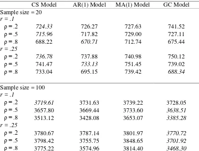
growth curve model sometimes did not have the lowest average AIC and BIC when it was the true model. Table 4 shows the average AIC of the four models when fitted to data simulated

with an RC structure, effect size of 0.5. The lowest AIC values among the four models were

italicized. We did not include BIC in the table because these two fit indices showed the

same pattern. As we can see from Table 4, the growth curve model, on average, was not

necessarily the best fitting model when the sample was small and when sample size = 100, r

= 0.1, and ρ = 0.2.

[TABLE 4 ABOUT HERE]

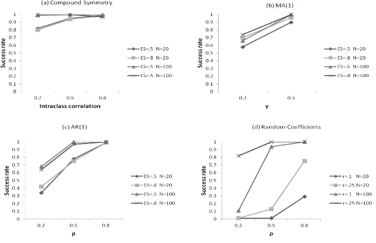
We then looked at the number of times the true model was selected by AIC and BIC

out of 100 comparisons. Figure 3(a) shows the success rates of AIC in selecting the

ANOVA model with different simulation values. We do not present the success rates of BIC

because they were almost identical to those of AIC (the same apply hereinafter). As

indicated in Figure 3(a), AIC and BIC performed very well when the true error structure was

were both small. Yet, even in the worst scenario, they successfully picked the ANOVA

model approximately 80% of the time. As ICC and sample size increased, the success rates

quickly improved to more than 90%.

[FIGURE 3 ABOUT HERE]

For data simulated to follow an AR(1) or MA(1) error structure, the success rate of

AIC and BIC was less satisfactory. As shown in Figure 3(b), when γ was small, AIC and

BIC correctly picked the MA(1) model 58% to 78% of the time, with a higher percentage

corresponding to a larger sample size. These numbers increased to more than 90% when γ

increased to 0.5. The same pattern was found for the AR(1) structure. As shown in Figure

3(c), AIC and BIC had the lowest success rates in selecting the AR(1) model when ρ was

small and sample size was small -only about 40%. When ρ was small but the sample size

increased to 100, the numbers increased to about 65%. If we increased both the value of ρ

and the sample size, AIC and BIC would have success rates close to 100%.

For data with an RC error structure (Figure 3(d)), AIC and BIC were less successful

when the sample size was small, with the smallest success rate occurring when either ρ (the

ratio of σi2 over the sum of σε2 and σi2) or r (the ratio of σs2 over σi2) was small. The success

rate increased slightly as ρ and r had larger values, but they were still very low in most cases (8% to 29%). The only exception was when ρ = 0.8 and r = 0.25, where the success rates reached approximately 70%. A sample size of 100 improved the performance of AIC and

BIC substantially. In most cases, the growth curve model was correctly chosen.

The performance of AIC and BIC seemed to be influenced by the similarity between

which alternative model AIC and BIC picked over the true model. For example, an AR(1) structure with a small ρ was very closed to CS and MA(1), thus, when it represented the true

model, AIC and BIC tended to wrongly pick the ANOVA model or the MA(1) model. If the

alternative structure was more parsimonious than the true structure, it became even more

difficult for AIC and BIC to identify the true structure. For instance, when the true structure

was RC and ρ and r were small, σi2 and σs2 would both be small. In this case, the variance

and covariance would change slowly, showing a pattern that resembled CS and AR(1).

Moreover, CS and AR(1) were more parsimonious than RC because they required fewer

parameter estimates. As a result, AIC and BIC tended to choose the ANOVA model or the

AR(1) model instead of the growth curve model. The problem was exacerbated when we

had a small sample size, that is, when few data were available for estimating the parameters.

In this case, AIC and BIC could hardly distinguish between these structures.

Comparing the Best Fitting ANOVA or Covariance Pattern Model to the Blanket

Selection of the Linear Growth Curve Model

In this section we are interested in considering the cost of selecting the wrong model.

How does that affect the inference? Does the model selected by AIC and BIC yield

statistical inferences that are similar to the true model? Does selecting the best fitting model

enhance our ability to make valid statistical inferences (in particular compared to the blanket

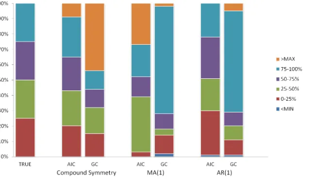
selection of the linear growth curve model)? To answers these questions, we examined the

tail probabilities (p-values) of the linear time effect of the best fitting ANOVA or covariance

pattern model to that of the growth curve model. For ANOVA and the covariance pattern

growth curve model, we used the linear slope. To compare them with the true model, we

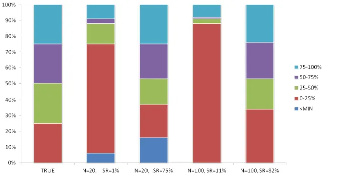
extracted the minimum (MIN), maximum (MAX), and the three quartiles (25%, 50%, 75%)

from the distribution of p-values of the linear time effect produced by the true model. We

then looked at the distribution of tail probabilities for the best fitting model and the growth

curve model by counting the frequencies of p-values they produced in each of the ranges

defined by those numbers (< MIN, 0 - 25%, 25 - 50%, 50 - 75%, 75 - 100%, and > MAX).

Because we were most concerned about the situations where AIC and BIC failed toidentify

the true model, we plotted these distributions for scenarios in which the success rates of AIC

and BIC were the lowest. As shown in Figure 4, the distribution of tail probabilities produced by the model selected by AIC (as well as BIC, which gave identical results) was

much closer to the true model6 than the growth curve model, for which the distribution of tail

probabilities concentrated at the higher end. This indicates that the blanket selection of the

growth curve model tends to yield higher p-values for the linear time effect and thus has a

lower power. In this case, using AIC and BIC to select the error structure for the data lowers

the risk of making a Type II error.

[FIGURE 4 ABOUT HERE]

Next, we looked at the distribution of tail probabilities of the linear time effect for the

best fitting model when the growth curve model is the true model. We plotted four

scenarios in Figure 5. We see that when the success rate was low, the model with the lowest

AIC tended to underestimate the p-value, regardless of the sample size. The results were

6

Note that this figure shows the distribution when the success rates of AIC and BIC were the lowest. With

similar for BIC. This suggests that when the fit indices fail to identify the growth curve

model as the true model, the Type I error rate may be inflated. When the success rate was

high, the distribution of the p-values produced by the best fitting model approached that of

the true model.

[FIGURE 5 ABOUT HERE]

Discussion

In this study, after using two real data examples to suggest that more than just the

growth curve model should be considered when answering certain questions relating to

change over time, we used simulation data to examine whether we can rely on AIC and BIC

to select the residual covariance structure for longitudinal data, given that the fixed effects

model is correct. Our results show that when sample size is not small, AIC and BIC

generally identify the true error structure. However, when sample size is small, AIC and

BIC may pick an alternative model that is similar to the true model. These results can be

compared with other simulation studies. Ferron et al. (2002) showed that in the presence of

hybrid error structures (e.g., a combination of RC and AR(1)), AIC and BIC may have

difficulty selecting the correct model. Wolfinger (1996) showed that when choosing

between two structures where the true structure is somewhere in between, the more

parsimonious structure may lead to more efficient inferences. Keselman et al. (1999)

showed that with small samples and relatively indistinguishable covariance structures (e.g.

ARH and RC), AIC and BIC perform less well than expected. Here with the more

qualitatively different structures, we see that for CS, MA(1) and AR(1), AIC and BIC

certain circumstances. The strict functional pattern of heterogeneity required for the

variances and covariances seems to be difficult to realize in the data. In this case, AIC and

BIC seem to be following Wolfinger’s (1996) suggestion that, when choosing between two

models that do not precisely fit the data, the more parsimonious model is the preferable

structure.

When the underlying error structure is CS, MA(1), or AR(1), the best fitting model

selected by AIC and BIC produces tail probabilities that are much more similar to the true

model than those produced by the linear growth curve model. However, the tendency of

AIC and BIC to choose a more parsimonious model when the true error structure is RC may

lead to an inflated Type I error. These results suggest that we should not use AIC and BIC for the selection of covariance model when the sample size is small. When the sample size

is not small, AIC and BIC seem to be able to distinguish among the different structures and

thus appear to be valid criteria for model selection.

The comparison of tail probabilities of the linear time effect reveals the potential

problem of the blanket selection of the linear growth curve model. Even when the means

fall onto a straight line, fitting a linear growth curve model can result in incorrect statistical

inferences when the data do not conform to the pattern that this model implies. This is also

demonstrated in the real data examples. An important assumption of the growth curve

model is that all individuals follow the same “growth” pattern. When this assumption is

violated, fitting the growth curve model may result in less power (as shown in the simulation

study) or an inflated Type I error rate (as in the job satisfaction example). Even when all

strict pattern that the growth curve model assumes, as in the strength training example. In

this case, the growth curve model may still not be the best model for the data. Meanwhile, it

should be noted that the linear growth curve model with random intercept and slope is not the

only option we have for conducting growth curve analysis. In this paper, we concentrate on

the case where both X and Z matrices contain only linear effects. It is possible and often necessary to include higher order polynomial effects or even nonlinear effects of time if the

change of a psychological construct follow a more complicated trajectory (McArdle &

Nesselroade, 2002; Ram & Grimm, 2007). Simply stated, the straight line may not

represent the correct means model for the data. Moreover, the effects that are included in Z

do not need to match those included in X. Even with a straight line means model, some alternative error covariance structure may better represent the data. When dealing with real

data, researchers should fully consider these options once they decide that growth curve

analysis is the method of choice.

To help researchers make sounder decisions in longitudinal data analysis, we

provide some practical guidelines for model selection. We limit our discussion here on

situations where the purpose of the analysis is to model mean differences in the response

variables which are assumed to follow a multivariate normal distribution. The first step is to

determine what options we have. If the data are from a repeated measures design that is

balanced on time, meaning that all individuals in the sample are supposed to be measured on

the same occasions, we have the flexibility to choose from among all three types of models.

This is true even when there are missing data. If we are dealing with data from a design that

we use age as the predictor), growth curve modeling is often the best option. In the case in

which all three models can be used, the next step will be to look at the mean pattern. In the

absence of the intention to test strong initial hypothesis regarding the means, we can conduct

exploratory analysis (e.g. a spaghetti plot or a breakdown of polynomial trend scores) to

examine whether the means and individual data follow a particular shape (e.g., straight line,

quadratic trend, etc.). If the sample shows substantial homogeneity, such that all individuals

seem to share the same pattern of “growth”, it will be reasonable to fit a growth curve model.

However, if the sample is heterogeneous in terms of developmental trajectories, the growth

curve model is not likely to be a good model.

Given a particular means model, we then need to determine a proper model for the

covariance matrix of the residuals (the error structure). Our simulation study suggests that

with a reasonable sample size, AIC and BIC are able to correctly select the error structure.

What could be deemed a “reasonable sample size” seems to depend on the covariance pattern

of the data. In our study, we only looked at sample sizes of 20, 100, and 200, and a sample

size of 100 is sufficient in most cases with various effect sizes and simulation values.

However, a smaller sample size (e.g., N=50) may be sufficient if the covariance matrix of the

data clearly conforms to a particular pattern. In the situation where the underlying pattern is

somewhat ambiguous and lies in between multiple structures, a larger sample size may be

needed. The bottom line is that fitting only one model and assuming that it adequately

describes the pattern of covariation in the data is rarely a good idea. Comparing different

error structures using AIC and BIC increases our chance of making a valid statistical

The current literature does not provide a clear answer as to how many and which error

structures we need to compare. We recommend starting with the unstructured pattern (i.e., a

saturated covariance model) because it does not make any assumptions about the population.

In this respect, it is the safest option. It also provides us with a useful diagnostic. The

model estimated with this structure will give us the covariance matrix of the residuals. This

can give us an indication of what other structures might be tenable. However, the

unstructured pattern may estimate too many parameters, especially when the number of

occasions is large. This may lead to a lower power (Wolfinger, 1996). Hence, other

structures need to be considered. The structures presented in our simulation study are

among those typically used in the analysis of repeated measures data. Besides, while higher

order autoregressive structures might be considered (such as AR(2)), the Toeplitz (or banded)

structure is a general autoregressive model that is often appropriate for longitudinal data.

Unlike AR(1), the Toeplize structures places no functional constraints on the autocorrelations

and thereby is less restrictive. Given the requirements of homogeneous variances for the

structures mentioned (except for the RC structure), heterogeneous versions of these structures

may also be considered.

In the event that the proper means model is to be determined empirically, the selection

of the covariance structure of the residuals becomes tied to each step of the process. For

example, if we are adding polynomial terms hierarchically in a growth curve model, the

inference related to the highest order polynomial term (i.e. whether that term is necessary) is

dependent on the error structure for that step. Methods such as the hierarchical

In our examples, we looked at different error structures under a common straight line

fixed effects means model. When comparing different models with not only different error

structures, but different means structures, the AIC and BIC should be constructed based on

the ML estimator, which, unlike the REML estimator, includes information and a parameter

count related to the fixed effects of the model (Verbeke & Molenberghs, 2000). The

definition of the comparative fit indices including information criteria for ML are described

in Littell et al. (2006).

The selection of the means model represents just one of the decisions we need to

make when selecting an analytic strategy to model fixed effects. Given the decision to treat

time as categorical and use ANOVA, one would then have the choice of omnibus testing and

follow-up contrasts contingent on significant main or interaction effects versus a set of

planned comparisons. For example, under the hypothesis that the means follow a straight

line, one could test a linear contrast. Under certain conditions (e.g. individuals measured at

the same occasions), the significance test of the linear contrast is equivalent to the

significance test of the average slope in a linear growth curve model (Maxwell & Delaney,

2004). The choice of omnibus testing/follow-up contrasts versus planned contrasts also

holds for the covariance pattern model. It is well known that under the correct hypothesis,

the planned contrast is a more powerful test than the omnibus test. More complete

discussions of the decisions related to the ANOVA approach appear in Hertzog & Rovine

(1985), Maxwell & Delaney (2004) and Stevens (1980).

In the ANOVA literature, it is well documented that violation of the sphericity

covariance matrix of residuals using alternative structures as suggested in this paper is one

way to insure proper statistical inferences when sphericity is violated. An alternative

method is to adjust the F-test based on a reduction of the error degrees of freedom

(Greenhouse & Geisser, 1959; Huynh & Feldt, 1970). Regardless of the method, contrasts

(either planned or follow-up) can be used to identify mean differences. Boik (1981) has

shown that both the omnibus ANOVA F-test and the contrasts based on the pooled mean

square error result in substantial bias. As a result he suggests a tailored contrast error term

for ANOVA-based contrasts. Similar tailored error terms are recommended and typically

provided in the linear mixed model software for contrasts based on the alternative error

structures described here (Littell et al., 2006). In this study we did not compare adjustments

to the ANOVA F-tests under violation of the sphericity assumption to the F-tests based on

alternative error structures, leaving the question open as to how the adjusted test would

compare to the alternative structure test. We also left the comparison between contrast

F-tests based on tailored error terms under compound symmetry (Boik, 1981) to contrast

F-tests based on tailored error terms under other structures for some later time.

While we dealt primarily with simple designs in this study, we could easily extend the

design by adding additional factors (Littell et al., 2006; Milliken & Johnson, 2009). The

approach to modeling the time-related factor would not change in the presence of additional between effects factors. In the linear mixed model approach, time effects are essentially

treated as specially constructed dependent variables (Hertzog & Rovine, 1985). Additional

repeated measures factors (e.g. family member) are treated by creating error covariance

for the other repeated measures factor.

In this study we use AIC and BIC as the fit indices, which do not provide information

on the absolute fit of the model. While in a structural equations modeling (SEM)

framework, we could test the fit of the model when data come from a balanced design (i.e.,

individuals are supposed to be measured on the same set of time points; Wu, West, & Taylor,

2009), in the mixed model framework relative fit indices such as AIC and BIC are the only

available options. So, while we can select the best-fitting model, it is not possible to tell

whether the best-fitting model is good enough, or, whether the other models fit the data

sufficiently well. An accompanying problem of this approach is the way in which the

relative fit indices are used. Since we need the fixed effect means model to generate the

residuals that are, then, modeled, we cannot uncouple the means model from the covariance

structure. In the SEM format we would first be able to fit the covariance structure and then

add the means model, an approach that is recommended in the SEM literature.

In the data examples and simulations we considered, the fixed effects model is a

straight line means model. Additional research is required to determine whether these

recommendations hold generally for more complex means models under a variety of

conditions.

In summary, based on the results of this study we think that the common practice of

fitting a linear growth curve model to repeated measures data without considering other

models may result in a less than optimal solution. The pattern that the growth curve model

poses on the covariance matrix should at least be compared with some alternative models.

model may not be optimal given the data. As a result, we recommend that, in addition to the

growth curve model, researchers consider the repeated-measures ANOVA and covariance

References

Akaike, H. (1974). A new look at the statistical model identification. IEEE Transactions on Automatic Control, 19(6), 716-723.

Bauer, D. J. (2003). Estimating multilevel linear models as structural equation models.

Journal of Educational and Behavioral Statistics, 28(2), 135-167.

Belsky, J., & Rovine, M. (1990). Patterns of marital change across the transition to

parenthood: Pregnancy to three years postpartum. Journal of Marriage and Family, 52, 5-19.

Biesanz, J. C., Deeb-Sossa, N., Papadakis, A. A., Bollen, K. A., & Curran, P. J. (2004). The

role of coding time in estimating and interpreting growth curve models. Psychological Methods, 9(1), 30-52.

Boik, R. (1981). A priori tests in repeated measures designs: Effects of nonsphericity.

Psychometrika, 46(3), 241-255.

Box, G., & Jenkins, G. (1970). Time Series Analysis: Forecasting and Control. San Francisco: Holden-Day.

Box, G. E. P. (1954). Some theorems on quadratic forms applied in the study of analysis of

variance problems, II: Effects of inequality of variance and of correlation between

errors in the two-way classification. Annals of Mathematical Statistics, 25, 484-498. Bryk, A. S., & Raudenbush, S. W. (1992). Hierarchical Linear Models. Newbury Park: Sage. Cohen, J. (1988). Statistical Power Analysis for the Behavioral Sciences (2nd ed.). Hillsdale,

Curran, P. J., & Bauer, D. J. (2007). Building path diagrams for multilevel models.

Psychological Methods, 12(3), 283-297.

Ferron, J., Dailey, R., & Yi, Q. (2002). Effects of misspecifying the first-level error structure

in two-level models of change. Multivariate Behavioral Research, 37(3), 379-403. Gelman, A., & Hill, J. (2007). Data Analysis Using Regression and Multilevel/Hierarchical

Models: Cambridge University Press.

Goldstein, H. I. (1995). Multilevel Statistical Modeling. London: E. Arnold.

Granger, C. W. J., & Morris, M. J. (1976). Time series modelling and interpretation. Journal of the Royal Statistical Society. Series A (General), 139(2), 246-257.

Greenhouse, S. W., & Geisser, S. (1959). On methods in the analysis of profile data.

Psychometrika, 24(2), 95-112.

Hartley, H. O., & Rao, J. N. K. (1967). Maximum-likelihood estimation for the mixed

analysis of variance model. Biometrika, 54, 93-108.

Harville, D. A. (1977). Maximum likelihood approaches to variance component estimation

and to related problems. Journal of the American Statistical Association, 72(320-340). Hedeker, D., & Gibbsons, R. D. (2006). Longitudinal Data Analysis. Hoboken, New Jersey:

John Wiley & Sons.

Henderson, C. R. (1953). Estimation of variance and covariance components. Biometrics, 9, 226-252.

Henderson, C. R. (1990). Statistical methods in animal improvement: Historical overview. In

Hertzog, C., & Rovine, M. (1985). Repeated-measures analysis of variance in developmental

research: Selected issues. Child Development, 56, 787-809.

Huynh, H., & Feldt, L. S. (1970). Conditions under which mean square ratios in repeated

measurements designs have exact F-distributions. Journal of the American Statistical Association, 65(332), 1582-1589.

Jennrich, R. I., & Schluchter, M. D. (1986). Unbalanced repeated-measures models with

structured covariance matrices. Biometrics, 42, 805-820.

Keselman, H. J., Algina, J., Kowalchuk, R. K., & Wolfinger, R. D. (1999). A comparison of

recent approaches to the analysis of repeated measurements. British Journal of Mathematical and Statistical Psychology, 52, 63-78.

Kwok, O.-M., West, S. G., & Green, S. B. (2007). The impact of misspecifying the

within-subject covariance structure in multiwave longitudinal multilevel models: A

Monte Carlo study. Multivariate Behavioral Research, 42(3), 557-592.

Laird, N. M., & Ware, J. H. (1982). Random-effects models for longitudinal data. Biometrics, 38, 963-974.

Littell, R. C., Milliken, G. A., Stroup, W. W., Wolfinger, R. D., & Schabenberger, O. (2006).

SAS for Mixed Models. Cary, NC: SAS Institute, Inc.

Maxwell, S. E., & Delaney, H. D. (2004). An introduction to multilevel models for

within-subjects designs. In S. E. Maxwell & H. D. Delaney (Eds.), Designing Experiments and Analyzing Data: A Model Comparison Perspective. Mahwah, NJ: Lawrence Erlbaum Associates.

data. Annual Review of Psychology, 60(1), 577-605.

McArdle, J. J., & Nesselroade, J. R. (2002). Growth curve analysis in contemporary

psychological research. In J. Schinka & W. Velicer (Eds.), Comprehensive Handbook of Psychology (Vol. 2, pp. 447-480). New York: Wiley.

McQuarrie, A. D. R., & Tsai, C.-L. (1998). Regression and Time Series Model Selection: World Scientific.

Milliken, G. A., & Johnson, D. E. (2009). Analysis of Messy Data, Volume 1-Designed Experiments: Chapman & Hall/CRC.

Myers, J. L. (1979). Fundamentals of Research Design. New York: Allyn and Bacon. Ram, N., & Grimm, K. (2007). Using simple and complex growth models to articulate

developmental change: Matching theory to method. International Journal of Behavioral Development, 31(4), 303-316.

Rao, C. R. (1958). Some statistical methods for the comparison of growth curves. Biometrics, 14, 1-17.

Robinson, G. K. (1991). That BLUP is a good thing: The estimation of random effects.

Statistical Science, 6(1), 15-51.

Rosenberg, B. (1973). Linear regression with randomly dispersed parameters. Biometrics, 60, 61-75.

Rovine, M. J., & Molenaar, P. C. M. (1998). The covariance between level and shape in the

latent growth curve model with estimated basis vector coefficients. Methods of Psychological Research Online, 3(2).

random coefficients model. Multivariate Behavioral Research, 35(1), 51-88.

Rovine, M. J., & Molenaar, P. C. M. (2005). Relating factor models for longitudinal data to

quasi-simplex and NARMA models. Multivariate Behavioral Research, 40(1), 83-114.

Schafer, J. L. (1997). Analysis of Incomplete Multivariate Data: Chapman & Hall/CRC. Scheffe, H. (1959). The Analysis of Variance. New York: Wiley.

Schwarz, G. (1978). Estimating the dimension of a model. Annals of Statistics, 6(2), 461-464. Singer, J. D., & Willett, J. B. (2003). Applied Longitudinal Data Analysis: Modeling Change

and Event Occurrence. New York: Oxford University Press.

Stevens, J. P. (1980). Power of the multivariate analysis of variance tests. Psychological Bulletin, 88(3), 728-737.

Tucker, L. R. (1958). Determination of the parameters of a functional relation by factor

analysis. Psychometrika, 23(1), 19-23.

Verbeke, G., & Molenberghs, G. (2000). Linear Mixed Models for Longitudinal Data. New York: Springer.

Wolfinger, R. D. (1996). Heterogeneous variance: Covariance structures for repeated

measures. Journal of Agricultural, Biological, and Environmental Statistics, 1(2), 205-230.

Wu, W., West, S. G., & Taylor, A. B. (2009). Evaluating model fit for growth curve models:

Table 1

Parameters Estimates, AIC and BIC from Models of Job Satisfaction, Various Error Structures

GC CS AR(1) TOEP MA(1) CSH ARH(1) TOEPH UN

Table 2

Distribution of Orthonormalized Polynomial Trend Scores

Job Satisfaction Weight Lifted

Linear trend score

Mean -0.96 0.72

Variance 14.30 1.61

Skewness -1.56 -0.01

Kurtosis 3.18 -0.08

Quadratic trend score

Mean -0.54 -0.12

Variance 8.93 0.48

Skewness -0.31 0.54

Kurtosis 2.92 0.16

Cubic trend score

Mean -0.41 0.11

Variance 4.79 0.33

Skewness -0.29 0.17

Kurtosis 0.77 0.35