Beta distribution

(1)

Beta Distribution

Paul Johnson <pauljohn@ku.edu> and Matt Beverlin <mbeverlin@ku.edu>

June 10, 2013

1 Description

How likely is it that the Communist Party will win the next elections in Russia?

In my view, the probability is 0.33. You may think the chance is 0.22. Your brother thinks the chances are 0.6 and his sister-in-law thinks the chances are 0.1.

People disagree and we would like a way to summarize the chances that a person will say 0.4 or 0.5 or whatnot.

The Beta density function is a very versatile way to represent outcomes like proportions or probabilities. It is defined on the continuum between 0 and 1. There are two parameters which work together to determine if the distribution has a mode in the interior of the unit interval and whether it is symmetrical.

The Beta can be used to describe not only the variety observed across people, but it can also describe your subjective degree of belief (in a Bayesian sense). If you are not entirely sure that the probability is 0.22, but rather you think that is the most likely value but that there is some chance that the value is higher or lower, then maybe your personal beliefs can be described as a Beta distribution.

2 Mathematical Definition

The standard Beta distribution gives the probability density of a value x on the interval (0,1):

Beta(α, β) : prob(x_|α, β) = x

α−1(1−x)β−1

B(α, β) (1)

where B is the beta function

B(α, β) =

Z 1

0

tα−1(1−_t)β−1_dt

2.1 Don’t let all of those betas confuse you.

It is disappointingly confusing, but the word “beta” is used for 3 completely different mean-ings.

1. Beta(α, β) “Beta” is the name of the probability distribution

(2)

2. B(α, β) “Beta” is the name of a function that appears in the denominator of the density function

3. β “Beta” is the name of the second parameter in the density function

2.2 About the Beta function

B

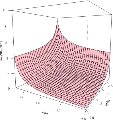
The Beta function B in the denominator plays the role of a “normalizing constant” which assures that the total area under the density curve equals 1.

The Beta function is equal to a ratio of Gamma functions:

B(α, β) = Γ(α)Γ(β) Γ(α+β)

Keeping in mind that for integers, Γ(k) = (k₋1)!, one can do some checking and get an idea of what the shape might be.

A 3 dimensional graph of the Beta function can be found in Figure 1.

3 Moments of the Beta

The expected value of a variable that is Beta distributed is:

E(x) =µ= α

α+β (2)

and the variance is

V ariance(x) = αβ

(α+β)2

(α+β+ 1) (3)

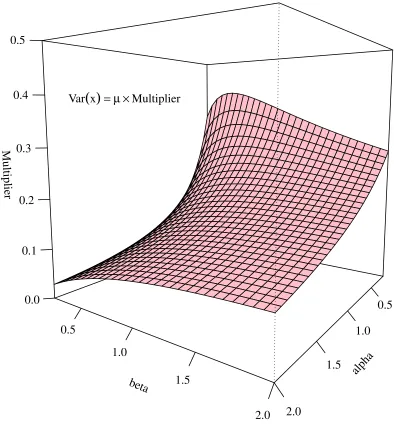
People who are familiar with the Generalized Linear Model will notice that

V(µ) = β

(α+β)(α+β+ 1)·µ

is a variance function, V(µ), which indicates the dependence of the observed variance on the mean. For a fixed pair of parameters (α, β), the variance is proportional to µ. A graph illustrating the Variance function is presented in Figure 2.

The third and fourth moments are:

(3)

alpha 0.5

1.0

1.5

2.0

beta

0.5

1.0

1.5

2.0

Beta Function

0 2 4 6 8 10

(4)

alpha 0.5

1.0

1.5

2.0 beta

0.5

1.0

1.5

2.0

Multiplier

0.0 0.1 0.2 0.3 0.4 0.5

Var

(

x

)

= µ ×Multiplier

(5)

0.0 0.2 0.4 0.6 0.8 1.0

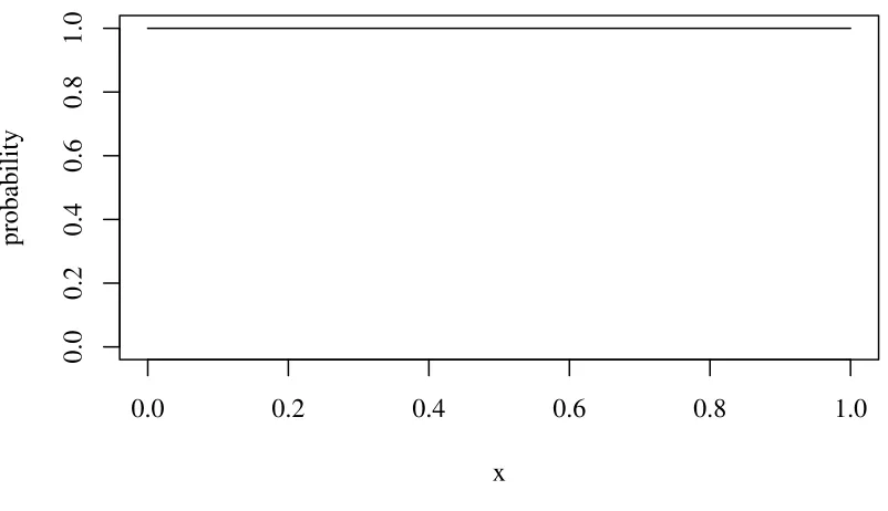
Figure 3: Beta(1,1) is the Uniform distribution

3.1 The Mode

As we will illustrate below, if α=β= 1, then the Beta is identical to a Uniform distri-bution.

4 Illustration

One advantage of the Beta distribution is that it can take on many different shapes. If one believed that all scores were equally likely, then one could set the parameters α= 1 and

β= 1, as illustrated in Figure 3, this gives a “flat” probability density function.

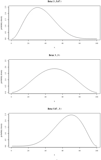
In models of elections, one may need a distribution of ideal points to resemble a single-peaked distribution on the interval [0,1]. The Beta can be very useful in this kind of exercise. Consider Figure 4.

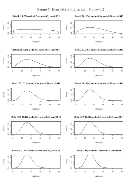
At one point, it fascinated me that the mode did not equal the mean and that the variance ends up characterizing the “slack” between those two things. Various densities in Figure 5 might be entertaining. In these examples, the Beta parameters are chosen to keep the mode constant at 0.3. Note how the mean and variance change across the illustrations.

(6)

0 20 40 60 80 100

(7)

Figure 5: Beta Distributions with Mode=0.3

0 20 40 60 80 100

0.0

1.5

3.0

Beta(1.1, 1.23) mode=0.3 mean=0.47, var=0.075

ideal point

Beta(7, 15) mode=0.3 mean=0.32, var=0.009

ideal point

density

(8)

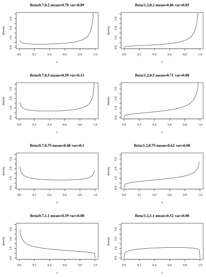
Perhaps, as they say, the versatility of the Beta is a strength, but there is some reason to be cautious. If the parameters wander into the (0,1) range, then some pretty surprising shapes can appear. Consider Figure 6.

5 About the connection between the mean, the mode,

and the variance

In the pictures displaying the Beta density, one’s eye is drawn to the peak of the frequency distribution, which is the mode. We can set the Beta’s parameters in order to generate a distribution with a desired mode. Let the mode be represented by γ.

Here’s a simple starting point: Suppose the mode is .50. That is the same as the mean (its symmetric), and the mode formula (6) implies:

.50 = α−1

If one wants the mode to be in the middle, one can choose any value for α,as long as one chooses the same value for β. (Whew! What a relief. This exactly matched my intuition.)

If the mode is in the center, we know α and β are equal, but we don’t know their

values. The selection, it turns out, depends on how much diversity there is. If one wants a distribution to have points “tightly bunched” around the mode, then one should choose a large value for α, say 10.0,

variance of Beta(10,10) = 0.01190 (9)

In contrast, if α= 1.5, the variance is much greater:

variance of Beta(1.5,1.5) = 0.0625 (10)

Seen in this light, the parameter α is a “homogeneity indicator.” As α gets bigger, the distribution collapses around the mode.

Although this particular calculation works only for a mode in the center, it does outline the process that we can use to assign α and β for all other values of the mode.

Suppose the mode is .4. From equation 6

.40 = α−1

α+β₋2

(9)

0.0 0.2 0.4 0.6 0.8 1.0

Figure 6: Some Unpleasant Betas

(10)

.40α+.40β₋0.8 =α₋1

It is quite possible to calculate one parameter as a function of another, after specifying the mode, even if the mode is off center.

Generally speaking, for any value of the mode, γ _∈(0,1) (keeping in mind the original stipulation that α, β >1):

γ= α−1

So α is a linear function of β. (Note: 2013-10-25; reader notified me of typographical error in equation 16. Sorry!)

And

This indicates that if we begin with the mode, and then take as given either α orβ, we can calculate the missing parameter (β or α, as the case may be). As a result, instead of thinking of the Beta’s shape as determined by parametersα and β, sometimes it is easier to think of it in terms of the mode (most likely value) and the homogeneity.