Analysis of Factors Affecting Unemployment in
Indonesia in 1984-2013
Nano Prawoto, P.hd
Lecturer at the Faculty of Economics,
University of Muhammadiyah Yogyakarta Indonesia
Email : [email protected]
ABSTRACT
The problem of unemployment is a very complex problem that is experienced by each developing country. In the macro economy, unemployment became the fundamental problems in both the short and long term. Indonesia is a country with a high population, Indonesia is the 4th after India although Indonesia has an abundance of natural resources. This should make the economy and economic growth in Indonesia increased. However, in fact, many Indonesian people do not have jobs or in other words become unemployed. This study aims to determine the factors that affect unemployment in Indonesia. Then the independent variables used are population, GDP, and interest rates, while the dependent variable is unemployment. In this paper, an analysis tool used is regression analysis Vector Error Correction Model (VECM). The analysis showed that the interest rate and the number of population statistically significant affect unemployment. R-Squared results show that the above variables affects as much as 76% and the remaining 24% is influenced by other variables outside the model. So that the interest rate and the number of the population affect unemployment.
Keywords: Unemployment, Population, interest rate, and the Gross Domestic Product.
A. Background
The problem of unemployment is a very complex problem that is experienced by each developing country. In the macro economy, unemployment became the fundamental problems in both the short and long term. Indonesia itself is a country that possess the number of people who are very much evident with Indonesia is ranked fourth after India and Indonesia itself has an abundance of natural resources. This should make the economy and economic growth in Indonesia increased. However, the fact now, many Indonesian citizens who do not have jobs or otherwise be unemployed.
market will offer employment number that is higher than the amount of labor demand.
The unemployment problem itself becomes a difficult problem to solve, because Indonesia itself is still very limited employment, and population growth is growing every year, also high labor supply and the insufficient number of existing jobs. In 2014, Indonesia is in fourth position with a total population of 253,6 million.
In addition to the total population, while other indicators that affect unemployment is the Gross Domestic Product. GDP is determined by the desire of households, enterprises, and government to spend its earnings. A growing number of economic actors to shop a lot of goods and services will increase the company's sales. Output increased the company will have an impact on the increased use of labor factor, this causes will decrease unemployment.
Last indicator is the interest rate, is one of the causes of rising unemployment in Indonesia. Whereby when the interest rate increases, the possibility of inflation that causes the prices of goods and services in the market increases, then the whole industry and the company will reduce its cost of production, one of them is labor. So with the workforce reduction will increase unemployment and the Indonesian economy would deteriorate.
B. Scope of Problem
in economics, basically factors affecting unemployment pretty much. However, due to limited resources available, the discussion of the problem in this study only discusses the variables that affect unemployment in Indonesia: population, GDP, and interest rate. As for the data used are annual data 1990 -2013
C. Formulation of the Problem
1. What is the effect of the number of people on unemployment in Indonesia? 2. What is the effect of GDP on unemployment in Indonesia?
3. What Effect effect on unemployment rates in Indonesia?
D. Research Purposes
The purpose of this study was to test how much influence the number of population, GDP and the interest rate on the number of unemployment in Indonesia in 1984-2013.
E. Theoretical Basis
Various theories were put forward below is the basis for the formulation of hypotheses and grounding in doing research .In this foundation will be discussed on unemployment, population, and GDP subu interest.
Theory of Unemployment
1994). Unemployment may occur due to an imbalance in the labor market. This shows that the number labor supplied exceeds the quantity of labor demanded.
Arsyad 1997, stating that there is a close relationship between high levels of unemployment and poverty. For most people, who do not have a permanent job or just part-time has always been among the group of people who are very poor. People who work for payment fixed in the government and private sectors are usually included among the middle and upper class society. Anyone who did not have jobs is poor, while working in full is a rich man. Because sometimes there are workers who do not work in urban voluntarily seek work better and more appropriate to the level of education. They refuse jobs they feel inferior and they are doing that because they have other sources that can help their financial problems. People like this can be called unemployed but not necessarily poor. Likewise is, the number of individuals who may work full time per day, but still earn revenue slightly.
Unemployment is divided into three types based on the circumstances that cause, among other things:
1. frictional unemployment, ie unemployment caused by the actions of someone workers to leave work and seek better employment or in accordance with her wishes. Frictional unemployment is unemployment that is temporary due to their time constraints, information and geographic conditions between job applicants with a job application opener.
2. Structural unemployment, ie unemployment caused by structural changes in the economy such as deterioration of some of the factors of production so that production has decreased and workers are laid off. Structural unemployment is a state in which the unemployed are looking for jobs are not able to meet the requirements specified job opening. The more developed an economy of an area will increase the need for human resources that have better quality than before.
3. Unemployment conjuncture, ie unemployment caused by the excess and apply natural unemployment as a result of a reduction in aggregate demand.
GDP. The increase in unemployment tends to be associated with lower real GDP growth. When the unemployment rate increases, the real GDP is likely to grow more slowly or even fall. The relationship between the unemployment rate with the real GDP of the United States is based on Okun's Law for the years 1951-2000 can be formulated as follows:
ΔY / Y = 3% - 2x Δu
ΔY / Y is the real GDP change Δu is the change in the unemployment rate.
Relations with the total population of unemployed
Generally resident is any person domiciled or residing in the territory of a country in a long time. Haryanto (2013: 23) explains that the population represents the total of human or residents who occupy an area in a given time period. Malthus argued about the relationship between population, real wages, and inflation. When the worker population grows faster than food production, then real wages dropped, due to population growth led to the cost of living is the cost of food rose. When the real wage in the region is high, it will affect unemployment. when it happened an increase in real wages of a company will reduce the number of workers, while labor supply there is still high. When labor supply is higher of the labor demand there will be unemployment. This means that Malthus thought that there is a positive influence between unemployment and the number of people, a different opinion precisely stated by Emili Durkheim. He assumes that unemployment and the number of residents have a negative relationship. When the population then there will be increased competition everyone to further improve the education and skills they have. Thus everyone is vying for the job and will hit its high unemployment rate.
Interest Rate relationship with Unemployment
Framework of thinking
F. Hypothesis
The hypothesis is defined as an interpretation formulated and accepted for a while to be verifiable (M. Nazir, 1998). Once the framework above, this research can be made the following hypotheses:
1. Allegedly a total population affect Unemployment in Indonesia. 2. Suspected GDP affect the level of unemployment in Indonesia.
3. Anticipated interest rate affects the level of unemployment in Indonesia.
G. Method of collecting data
The data used in this study is data from the years 1984-2013. While the data collection methods used in this study is to collect data that is appropriate and relevant to the variables tested systematically in response to years of research from various sources are concerned, the main source of data collection are:
1. The Central Bureau of Statistics, Bantul, Yogyakarta 2. Development World Bank
H. Data analysis method
Corection Error Vector Model (VECM) is a derivative of the VAR. Assumptions need to be met as VAR, except statsioneritas problem. Unlike the VAR, VECM to be stationary at the first differential and all must have the same stationary, are differentiated in the first instance.
Prior to determining the right model separately using the data in this study. There are several steps that must be passed first, namely :
1. Stationarity Test Data
The economic data time series in general stochastic (trending is not stationary/data that have roots units). If the data has a unit root, then its value will tend to fluctuate around an average value, making it difficult to estimate a model. (Rusydiana, 2009). The unit root test is one concept that is increasingly population used to test stasioneran time series data. This test developed by Dickey and Fuller,
Unemploymen Population
GDP
using Augmented Dickey Fuller Test. Stationarity test to be used is ADF test using a 5% significance level.
2. Test the determination of lag
VAR model estimation begins by determining how long the lag is right in the VAR model. Determination of the optimal lag length is important in modeling VAR. If the optimal lag entered is too short it is feared could not explain the dynamism of the model as a whole. However, the optimal lag is too long will produce an estimated inefficient due to the reduced degree of freedom (especially models with a small sample). Therefore it is necessary to know the optimal lag before making estimates VAR.
3. Stability Test VAR
Var stability needs to be tested to determine the level of stability of data, if the results of the stability of the VAR estimation is not stable then the analysis of IRF and FEVD become invalid. Based on the test results of a VAR system is stable if the entire root or roots have the value of modulus smaller than one.
4. Test cointegration
Based on the lag length has been tested before, then proceed with the cointegration test to determine whether there will be a balance in the long term, that there are similarities between the movements of stability variables in the study or not. Cointegration test is performed to determine the existence of the relationship between variables, especially in the long term. If there is cointegration in variables used in the model means it can be ensured long-term relationship between the variables. In the study, cointegration tests are usually based using Johansen's Cointegration Test.
5. Granger Causality Test
Granger causality test is performed to determine whether an endogenous variable can be treated as an exogenous variable. This stems from ignorance of
VAR or VECM model test was conducted to determine the effect of long-term and short-term data from both independent and dependent. Whether there is a relationship in the short or long term of the independent variable on the dependent variable. If the results show more than plus or minus 2 it can be said that the independent variables have an effect on the dependent variable.
7. Test IRF (impulse response function)
propagators of the other variables and how long these effects occur. (Nugroho, 2009). Through IRF, the response an independent change of one standard deviation can be reviewed. IRF explore the impact of interference by one standard error (standard error) as innovations in one variable, it will directly impact on the relevant variables and then proceed to all other endogenous variables through the dynamic structure of the VAR.
8. Test Variance Decomposition
Variance decomposition aims to measure the magnitude of the contribution or influence the composition of each independent variable on the dependent variable. FEVD or forecast error variance decomposition innovation outlines a variable to components of other variables in the VAR or VECM. The information presented in FEVD are sequentially proportions movement caused by the shock itself an other variables.
I. Data analysis
From the results of research conducted by the authors obtain a test result based on the data that has been processed. Based on the results of the processing of data can be drawn between the analysis and discussion of the results is as follows:
1. Test Stationary
Variabel ADF T-Statistik
Nilai kritis
Prob
1% 5% 10%
Unemploymen -3.7736 -3.6891 -2.9718 -2.6251 0.0082
Population -5.0827 -3.6891 -2.9718 -2.6251 0.0003
GDP -3.5451 -3.6891 -2.9718 -2.6251 0.0140
Interest -5.7364 -3.6998 -2.9762 -2.6274 0.0001
From the above table, one that is stationary test phase, in the stationary test shows that all four variables are stationary at 1st different (does not contain the root unit) for ADF t-value is less than the critical value MacKinnon. In addition, the value of probablitias passed since the probability value is below the critical value test is <1% (0:01) and interpret that data series are fit for use further testing to estimation of cointegration and VECM model for stationary use at the first difference
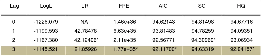
1. Test Long Lag
Table 2. Results of testing the optimal lag
Election results above optimal lag is expressed with a lag of three (3) based on the value of LR and FPE which coincides with the referenced value AIC. And lag 3 is recommended with more stars than lag 2.
2. Stability Test VAR
The third stage is test the stability of the VAR, in this test concluded that the estimated VAR stability that will be used for the analysis of IRF and FEVD has been and is in stable condition since the modulus value <1 (less than 1). The following table estimates or results of stability tests VAR.
Table 3. Stability VAR
Root Modulus
0.723155 0.723155
0.191064 - 0.663153i 0.690128
0.191064 + 0.663153i 0.690128
-0.547967 0.547967
-0.198242 - 0.336076i 0.390189
-0.198242 + 0.336076i 0.390189
0.248958 - 0.237244i 0.343896
0.248958 + 0.237244i 0.343896
No root lies outside the unit circle. VAR satisfies the stability condition.
3. Test Cointegration
The fourth stage is the Cointegration test is whether there is cointegration between independent variables with the dependent variable in the long run. According to the test results showed that the value of the trace statistics and maximum eigenvalue at r = 0 is greater than the critical value at significance level of 1% and 5%. There are two cointegration at a significance level of 1% and 5%, thus the results indicated that the co integration among the total population movements, interest rate, and GDP has a relationship stability / balance and
Lag LogL LR FPE AIC SC HQ
0 -1226.079 NA 1.46e+36 94.62143 94.81498 94.67716
1 -1199.593 42.78478 6.63e+35 93.81483 94.78259 94.09351
2 -1167.380 42.12406* 2.11e+35 92.56771 94.30969* 93.06934
equality movement in the long term. Here below is a table of test results cointegration.
Table 4. Cointegration Test Results
Hypothesized Trace 0.05
No. of CE(s) Eigenvalue Statistic Critical Value Prob.**
None * 0.808968 75.43596 47.85613 0.0000 At most 1 * 0.466308 32.39785 29.79707 0.0245 At most 2 * 0.402170 16.07152 15.49471 0.0409 At most 3 0.098492 2.695832 3.841466 0.1006
4. Granger Causality Test
Table 5. Granger Causality Test
Null Hypothesis: Obs F-Statistic Prob.
JP does not Granger Cause PENGANGGURAN 27 1.95227 0.1537 PENGANGGURAN does not Granger Cause JP 0.77503 0.5216
GDP does not Granger Cause PENGANGGURAN 27 0.68744 0.5702 PENGANGGURAN does not Granger Cause GDP 0.13397 0.9387
SB does not Granger Cause PENGANGGURAN 27 9.07011 0.0005 PENGANGGURAN does not Granger Cause SB 1.32326 0.2947
GDP does not Granger Cause JP 27 8.37996 0.0008
JP does not Granger Cause GDP 0.79725 0.5098
SB does not Granger Cause JP 27 7.30822 0.0017
JP does not Granger Cause SB 1.56353 0.2294
SB does not Granger Cause GDP 27 0.85858 0.4786
GDP does not Granger Cause SB 2.06157 0.1376
Note : PENGANGGURAN = Unemployment
SB = Interest Rate
JP = Population
GDP = Gross Domestic Product
1. SB variables (interest rate) was statistically significantly affect unemployment (0.0005), while not significantly influence the unemployment rate (0.2947). 2. Variable total population (JP) was statistically significantly affect GDP / GDP
3. SB variables (interest rate) was statistically significantly affect the total population (JP) (0.0017), while the total population (JP) did not significantly influence the SB (interest rate) (0.2294).
5. Test Model VECM
After testing granger causality, then will be tested the model VECM in this test determines there a relationship short term and long term between the variables Unemployment, Total population, interest rates and GDP where the dependent variable is unemployment, while the independent variable is the number of residents, interest rates, and GDP so VECM model estimation results of analyzing the effect of short-term and long-term dependent variable to the independent variables. The results of these estimates can be seen by the table below:
Variabel Koefisien t-Statistik
Cointeq1 -0.128902 [-1.75797]
D(PENGANGGURAN(-1),2) -0.423606 [-2.25043] D(PENGANGGURAN(-2),2 0.308414 [ 1.45567]
D(JP(-1),2) -0.049893 [-0.32490]
D(JP(-2),2) -0.279906 [-1.50392]
D(GDP(-1),2) -3.122170 [-2.97247]
(CGDP(-2),2) 0.367146 [ 0.41720] D(DSB(-1),2) -14109.50 [-0.23602] D(DSB(-2),2) -21090.61 [-0.48132]
C 36835.53 [ 0.31903]
R-Squared 0.768988
The estimation results indicate that the short term variable lag Unemployment in 3 to positive effect. This means that if there is an increase of 1% in the previous two years will increase unemployment by 0:42 percent in current year. If there is an increase of 1 per cent of total population in the two previous years, the decline in the unemployment rate to 0.279906 percent. If there is an increase of 1 percent of GDP in the first year before the decline in the unemployment rate to 3.122170 percent. This condition is consistent with the theory that when GDP/income rises it will reduce unemployment. R-Squared results show that the above variables affects as much as 76% and the remaining 24% is influenced by other variables outside the model.
Impact of Monetary Policy on Economic Growth in the Long Term
Variabel Coefisien t-statistik
D(GDP(-1)) 2.683539 [ 1.94105]
D(SB(-1)) 1366230. [ 8.74663]
In the long-term variable number of population, GDP and interest rates are significant at the five percent level that affect unemployment. Variable Population has a negative effect on unemployment is equal to -1.839435 percent, meaning that if there is an increase the number of people it will cause a decrease in the unemployment rate to 1.839435. GDP variable has a positive effect on unemployment is equal to -2.6835 per cent, meaning that if an increase in GDP will cause an increase in the unemployment rate to 2.6835 as well as the interest rate has a positive impact on unemployment in the amount of 1.36623 million percent which means is that if interest rates rise, it will cause 1366230 percent of the increase in unemployment.
6. Impulse Response Function (IRF)
Picture. IRF Test Results
-500,000 0 500,000 1,000,000 1,500,000
1 2 3 4 5 6 7 8 9 10
Response of D(BJP) to D(APENGANGGURAN)
The graph above shows the responses of the shock variable number of people unemployed. The shock of unemployment beginning to respond to the trend of negative (-) to enter the 3rd period. The response began to stabilize in the next period and start moving up into the period 10.
J. Conclusion
population (JP) (0.0017), while the total population (JP) did not significantly influence the SB (interest rate) (0.2294).
2. In the model VECM estimation results indicate that the short-term variable lag Unemployment in 3 to positive effect. This means that if there is an increase of 1% in the previous two years will increase unemployment by 0:42 percent in current year. If there is an increase of 1 per cent of total population in the two previous years, the decline in the unemployment rate to 0.279906 percent. If there is an increase of 1 percent of GDP in the first year before the decline in the unemployment rate to 3.122170 percent. This condition is consistent with the theory that when GDP / income rises it will reduce unemployment. R-Squared results show that the above variables affects as much as 76% and the remaining 24% is influenced by other variables outside the model.
3. In the long-term variable number of population, GDP and interest rates are significant at the five percent level that affect unemployment. Variable Population has a negative effect on unemployment is equal to -1.839435 percent, meaning that if there is an increase the number of people it will cause a decrease in the unemployment rate to 1.839435. GDP variable has a positive effect on unemployment is equal to -2.6835 per cent, meaning that if an increase in GDP will cause an increase in the unemployment rate to 2.6835 as well as the interest rate has a positive impact on unemployment in the amount of 1.36623 million percent which means is that if interest rates rise, it will cause 1366230 percent of the increase in unemployment.
4. The population's response to the shock variable unemployment. The shock of unemployment beginning to respond to the trend of negative (-) to enter the 3rd period. The response began to stabilize in the next period and begun moving up into the period 10.
K. SUGGESTION
1. The government's policy against unemployment and stressed again, especially in terms of labor supply. To avoid unequal distribution of income.
Reference
Agus Tri Basuki & Nano Prawoto, 2016, Analisis Regresi dalam Penelitian Ekonomi dan Bisnis, Penerbit RajaGrafido, Jakarta.
Ardiyanto, Danis.2012. Analisa Keterkaitan Pengeluaran Pemerintah dan Produk Domestic Bruto di Indonesia, Pendekatan Vector Error Corection Model (VECM).
Universitas Brawijaya 10 Juni 2013 Malang.
Alghofari, Farid. Analisis Tingkat Pengangguran di Indonesia. Universitas Diponegoro Semarang.
Abdune,Jonny. PENGARUH GROSS DOMESTIC PRODUCT, NILAI TUKAR, SUKU
BUNGA, DAN INFLASI TERHADAP PENANAMAN MODAL ASING DI
INDONESIA PERIODE2003.Q1–2012.Q.Universitas Brawijaya, Malang.
Gujarati, Damodar N. 2003. Basic Econometrics. 4th Edition. McGraw-Hill, New York, USA.
Lindiarta, Ayudha. Analisis pengaruh Tingkat upah Minimum, inflasi dan jumlah
penduduk terhadap tingkat pengangguran tahun (1996-2013). Universitas
Brawijaya di Malang 24 Juni 2013.
Sadono Sukirno, 1994. Pengantar Teori Ekonomi Makro. Penerbit RajaGrafindo, Jakarta
Sukirno, 2007. Ekonomi Pembangunan: Proses, Masalah, dan Dasar Kebijakan. Penerbit Kencana Prenada Media Group; Jakarta.
Tambunan, Tulus T.H. (2001), Perekonomian Indonesia : Teori dan Temuan Empiris, Ghalia Indonesia, Jakarta.
Utomo, Fajar Wahyu.2013. Pengaruh Inflasi dan Upah Terhadap Pe ngangguran di
Indonesia Periode tahun 1980-2010. Universitas Brawijaya Tanggal 5 April 2013