FORUM is intended for new ideas or new ways of interpreting existing information. It provides a chance for suggesting hypotheses and for challenging current thinking on ecological issues. A lighter prose, designed to attract readers, will be permitted. Formal research reports, albeit short, will not be accepted, and all contributions should be concise with a relatively short list of references. A summary is not required.
FORUM
FORUM
FORUM
Statistical significance
7
ersus fit
:
estimating the importance of
indi
7
idual factors in ecological analysis of
7
ariance
Michael H.Graham, Scripps Inst. of Oceanography, 9500 Gilman Dri7e MC 0208, La Jolla, CA 92093, USA
(present address: Center for Population Biology, One Shields A7e., Uni7. of California, Da7is, CA 95616, USA
[mhgraham@ucda7is.edu]. – Matthew S.Edwards,Dept of Ecology and E7olutionary Biology,Uni7.of California,
Santa Cruz,CA 95064,USA.
Although analysis of variance (ANOVA) is widely used by ecologists, the full potential of ANOVA as a descriptive tool has not been realized in most ecological studies. As questions ad-dressed by ecologists become more complex, and experimental and sampling designs more complicated, it is necessary for ecologists to estimate both statistical significance and fit when comparing the relative importance of individual factors in an explanatory model, especially when models are multi-factorial. Yet, with few exceptions, ecologists are only presenting signifi-cance values with ANOVA results. Here we review methods for estimating statistical fit (magnitude of effect) for individual ANOVA factors based on variance components and provide examples of their application to field data. Furthermore, we detail the potential occurrence of negative variance components when determining magnitude of effects in ANOVA and describe simple remediation procedures. The techniques we advocate are efficient and will greatly enhance analyses of a wide variety of ANOVA models used in ecological studies. Estimation of magni-tude of effects will particularly benefit the analysis of complex multi-factorial ANOVAs where emphasis is on interpreting the relative importance of many individual factors.
In contemporary ecology, realization of the inherent complexity of interactions among organisms and their environment typically leads to the design of compli-cated studies. Experimental ecologists often favor
elab-orate multi-factorial designs that simultaneously
investigate the main effects of many factors as well as their subsequent higher-order interactions (Underwood 1997). Recent studies have also shown that sampling and/or experimentation carried out at numerous hierar-chical scales of space and time can greatly enhance understanding of spatio-temporal variability in ecologi-cal processes (Connell et al. 1997, Karlson and Cornell 1998, Hughes et al. 1999). Fortunately, quantitative analysis of such multi-factorial data sets has been
facil-itated by a rich and well established statistical litera-ture, with general linear modeling techniques (e.g. multiple regression and multi-factorial analysis of vari-ance or ANOVA) finding considerable use in a variety of situations. The primary benefit of these analyses is that they can estimate the combined importance of all factors of interest, as well as compare the relative importance of individual factors and their interactions. When multi-factorial analyses are conducted primar-ily for the purpose of comparing the relative impor-tance of individual factors, sufficient conclusions often can be made from simple graphical plots of means and variances. As such, graphical analysis of multi-factorial data should always precede the use of inferential statis-tics. When patterns of multi-factorial data become con-fused, or when ecologists are reluctant to rely solely on graphical analyses, statistical significance and fit of individual factors can be determined relatively easily (Winer et al. 1991, Neter et al. 1996). The significance of a factor describes how likely (estimates the probabil-ity that) the patterns explained by the factor are simply due to random chance and thus serve no functional importance to the researcher. Significance is inherently dependent on the amount of data collected (sample size) and is typically presented in the form of probabil-ity-values (Pvalues). Conversely, determination of fit is not probabilistic, but rather is an estimate of the vari-ance in a response variable that can be explained by the factor. A factor’s fit is thus a measure of the magnitude of that factor’s effect on the response variable. Esti-mates of factor fit are usually termed ‘coefficients of determination’ (r2) in regression analyses and
‘magni-tude of effects’ (v2) in ANOVA (Winer et al. 1991,
factor’s fit is notdirectlydependent on sample size, and significance and fit do not necessarily co-vary. Conse-quently, the most significant factors in a multi-factorial analysis are not guaranteed to also have the greatest fit. Estimates of significance and fit can therefore be used to describe different aspects of statistical results.
Although ecologists have typically been diligent about reporting both factor significance and fit for regression analyses, they have with few exceptions ap-parently settled for describing ANOVA results by fac-tor significance alone. When using ANOVA to interpret results of ecological experiments, most ecologists have
simply presented P values as evidence of, or lack
thereof, the biological importance of some factor (e.g. competition or predation) on a response variable (e.g. growth or survivorship). We reviewed all issues of Australian Journal of Ecology, Ecology, Journal of Ecology, and Oikos published in 1998 and found that factor fit was estimated in only 2 of 184 (1.1%) papers that used ANOVA. By ignoring factor fit, researchers fail to utilize the full descriptive power of ANOVA, potentially leading to an incorrect interpretation of a factor’s ‘true’ biological importance. Factors that are highly significant, yet explain little variability in the response variable (low magnitude of effects), can result when sample sizes are simply large enough to detect statistically weak effects. Without determining magni-tude of effects, greater emphasis might be placed on the importance of such factors than is warranted. Further-more, it may be impossible to compare the relative importance of individual factors or interactions in a multi-factorial ANOVA when more than one factor is found to be significant but magnitude of effects are not presented. That is, researchers may be unable to distin-guish the effects of weak factors from strong ones. Given the potential presence of multiple significant factors of varied strength in ecological ANOVAs, and in ecology in general (Paine 1992, Berlow 1999), the description and interpretation of ecological data will be enhanced by the determination of both a factor’s sig-nificance and its fit.
We suspect that the primary reason ecologists fail to report magnitude of effects for individual factors in ANOVA is due to a lack of familiarity with the statisti-cal methodology for making such determinations. Such unfamiliarity is understandable given that many bio-statistical texts (e.g. Sokal and Rohlf 1981, Zar 1996) provide only brief (if any) descriptions of magnitude of effects, although a modest statistical literature on the subject does exist (e.g. Vaughn and Corballis 1969, Dodd and Schultz 1973, Winer et al. 1991, Searle et al. 1992, Neter et al. 1996, Underwood 1997). Here, we review the logic and methods for determining magni-tude of effects for individual factors in ANOVA. Our emphasis is primarily with multi-factorial ANOVAs, as these models will likely see the greatest benefit due to estimation of magnitude of effects. We further
demon-strate the utility of these methods by (1) applying them to real data for a variety of ANOVA models commonly used by ecologists and (2) providing published exam-ples of how the interpretation of ecological ANOVA is enhanced by the estimation of magnitude of effects. Our goal is to give the reader an overview of the methods and advantages of estimating the magnitude of effects, so that these estimates might be better inte-grated into the presentation of ANOVA results in ecological studies.
Determining magnitude of effects in ANOVA
We recognize two methods for estimating the relative importance of individual factors in ANOVA. The first, recommended by Weldon and Slauson (1986), estimates the ‘percentage contribution’ of a particular factor to the total sums of squares of a response variable. Al-though simple, this method is sensitive to differences in sample size and design (Underwood and Petraitis 1993) and does not attempt to isolate the ‘true’ effect of a factor from that of sampling variability (i.e. it ignores the composition of expected mean squares; see below). The second method estimates the relative magnitude of effects for individual factors in ANOVA by decompos-ing each factor’s mean square into its variance compo-nents. This method has been well described in the statistical literature (Vaughn and Corballis 1969, Dodd and Schultz 1973, Winer et al. 1991, Searle et al. 1992, Neter et al. 1996) and in some texts that emphasize the use of ANOVA in ecological studies (Underwood 1997). This method is more robust to variable sample sizes and sampling designs than that of Weldon and Slauson (1986) and will likely be of greater use to ecologists. Therefore, we favor this method for estimat-ing the relative importance of individual factors in ANOVA and devote the remainder of this paper to it. The basic logic for determining the magnitude of
effects (v2) for a factor in an ANOVA is simple:
expected mean squares (E{MS}) and are particular to each factor. Expected mean squares for most ANOVA models can be found in the statistical literature (see above references) or can be determined directly by the researcher (Searle et al. 1992, Underwood 1997). Exam-ples of calculated and expected mean squares for one-way, two-way (fixed, random, and mixed), and nested ANOVAs are given in Table 1, although we caution that the interpretation of expected mean squares will vary depending on whether they represent fixed or random variables (see Problems with magnitude of effects estimates). The formulae for expected mean squares should be familiar as they are used to specify the correctFratios for determination of factor
signifi-cance in ANOVA. Clearly, the complexity of expected mean squares is determined by the complexity of the ANOVA model, and the identification of proper ex-pected mean squares for a given model is not an insignificant task. The reader should refer to Winer et al. (1991) and Underwood (1997) for a more complete discussion on the determination of expected mean squares, especially for ANOVA models more compli-cated than those presented in Table 1.
Once expected mean squares have been determined for each factor in the ANOVA, a factor’s variance component (s2) can be isolated from the expected mean
squares by substitution and simple algebra. Variance components can be estimated for each factor and the
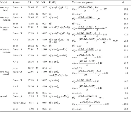
Table 1. Sums of squares, degrees of freedom, mean squares, expected mean squares (E{MS}), variance components, and magnitude of effects (v2, presented as percentages) for a variety of ANOVA models. Factor A was fixed for the two-way mixed model and random for the nested model. Data are the same for the two one-way ANOVAs and three two-way ANOVAs to allow comparisons of magnitude of effects among different models.a2equals the sums-of-squared deviations among factor levels, where factor A has levelsj=1 toJand factor B has levelsk=1 toK;nis the sample size within each level. Note that fixed effect variances (e.g.sA2=aj2/(J−1)) are converted to population variances (aj2/J) when calculating variance compo-nents (Vaughn and Corballis 1969, Winer et al. 1991).n=3 for all models;J=11 for one-way models, 3 for two-way models, and 2 for the nested model;K=5 for two-way models, and 2 for nested model. Data for one- and two-way models are from Graham (1999) and data for the nested model are from Edwards (unpubl.).
Source v2
Model SS DF MS E{MS} Variance component
10 Factor B 67.89 4 16.97
sB2=
nested 1 2.85 72.3
mean square error (s e
2) for most ANOVA designs
(Table 1). The estimation of variance components is an important step in ecological ANOVA because variance components are the best estimate of the contribution of a given factor to variability in a response variable. As such, variance components alone can be valuable de-scriptors of ANOVA results. If it is assumed that the total variability observed in a response variable is the sum of the variance components for all factors included in the model plus the mean square error (Vaughn and Corballis 1969, Dodd and Schultz 1973, Winer et al. 1991; but see concerns of Underwood 1997), then the relative (%) contribution of each variance component to the response variable (v2) can be estimated by
divid-ing each variance component by this total (Table 1). Furthermore, the sum ofv2for all factors included in
the model represents the variance in the response vari-able that can be explained by theo6erallmodel. Thus,
once the correct expected mean squares for an ANOVA model have been specified, calculation of the variance components and magnitude of effects for each factor (and the error) is relatively straightforward.
Problems with magnitude of effects estimates
Estimating the magnitude of effects in ANOVA is not without its problems. As previously stated, variance component estimates depend strongly on the correct identification of expected mean squares for the particu-lar ANOVA model being analyzed, and these expected mean squares may not be particularly intuitive when ANOVA models incorporate both fixed and random factors. The problem with ANOVA models that incor-porate both fixed and random factors revolves around the correct identification of the expected mean squares (see Table 1), as well as the appropriate interpretation of their meaning. The use of fixed versus random factors in ecological studies has been well-addressed (e.g. Potvin 1993, Bennington and Thayne 1994, New-man et al. 1997, Underwood 1997), and we therefore limit our discussion to the analytical and conceptual problems that pertain to estimating variance compo-nents and determining magnitude of effects.
Problems arise because of the inherent differences in underlying hypotheses relating to fixed and random factors. Fixed factors are those in which the factor levels examined in the analysis represent all levels of interest; the levels are imposed by the researcher and are generally of particular inferential importance. In contrast, random factors are those in which the factor
levels examined represent only a random subset of a
larger (infinite) population of factor levels; the levels are chosen simply to obtain an accurate estimate of the within-factor variance so that inferences can be drawn about the entire population from which levels were sampled. Although not always straightforward,
espe-cially in cases where factor levels represent differences in space or time, the correct identification of factors as being either fixed or random is essential to calculating magnitude of effects (see Table 1). The main problem is that random factors, through their interaction with other factors in the ANOVA model, are assumed to alter the expected mean squares of those factors. Since these interactions are estimated from only a subset of the random factor’s levels examined in the analysis, their variance contributions are not precisely known, thereby enhancing the uncertainty (variance) of the associated factors in the ANOVA model. In contrast, interactions with fixed factors are determined from all levels of those factors, as these are the sole levels under statistical and inferential investigation. The variance contributions of these interactions are therefore pre-cisely known and have little effect on the uncertainty of other factors in the ANOVA model. These analytical differences between fixed and random factors become apparent when comparing the calculation of expected mean squares for two-way fixed, random, and mixed ANOVA models (Table 1).
Once individual factors are identified as either fixed or random, the calculation of their variance compo-nents is relatively straightforward (see Table 1). How-ever, problems may arise if ANOVA models include two or more random factors. In this case, the precise calculation of some variance components may not be possible, much as the precise calculation of some F -statistics are not possible (Underwood 1997). Further-more, for ANOVA models that include only fixed factors, the choice of factor levels with similar effects on a response variable will result in smaller variance component estimates (and hence smaller magnitude of effects) than for factor levels with very different effects on the response variable. These problems can become further complicated when ANOVA models incorporate blocking factors, repeated-measures factors, or various degrees of nesting (Vaughn and Corballis 1969, Dodd and Schultz 1973, Winer et al. 1991, Underwood 1997). Conceptual and inferential difficulties can also arise if the researcher wants to compare magnitude of effects
betweenfixed and random factors (Underwood 1997). It is therefore vital that researchers carefully consider the identity and justification of factor levels before assign-ing them to experimental units.
stated that magnitude of effects estimated for individual factors using the above methodology are all determined
relati6e to the contributions of other factors in the
model and sampling error, and he questioned the rele-vance of such estimates. Comparisons of magnitude of effects among different experiments, and thus different ANOVAs, may be unreasonable since each analysis would have its own relative baseline (i.e. total variabil-ity in a response variable may vary among experi-ments). As Underwood (1997) acknowledged, such circumstances would limit comparisons of magnitude of effects towithina given experiment and it is important that the reader recognizes this constraint when calculat-ing and discusscalculat-ing magnitude of effects. In other words, if total variability is found to vary among different ANOVAs, then the importance of a given factor can only be determined relative to its baseline, and can therefore only be compared to other variables that use that same baseline. In such cases, variance component estimates are more appropriate than magnitude of ef-fects because they are not estimated relative to a base-line. If, however, it can be shown that total variability is similar for different experiments, among-experiment comparisons of magnitude of effects may be reason-able. Comparison of within- and among-experiment differences in the contribution individual ANOVA fac-tors may therefore be best done by presenting both absolute (variance components) and relative (magni-tude of effects) estimates.
A final problem with determining magnitude of ef-fects for individual factors in ANOVA is that negative variance components can be obtained from rearranging a factor’s expected mean square (e.g. the nested ANOVA example in Table 1). This is because variance component estimates are just as vulnerable to imprecise measurement as other statistical parameters; negative
variance components are analogous to F ratios B1.
Yet, negative variance components clearly violate the concept of variance. Although negative variance com-ponents can occur in any ANOVA model, we have found them to occur most often in nested designs (discussed below; Graham 1999, M. S. Edwards un-publ.). Winer et al. (1991) and Searle et al. (1992) both discuss the occurrence and potential remediation of negative variance components in ANOVA, and a few papers in the primary statistical literature specifically address this problem (Thompson 1962, Thompson and Moore 1963). Because ecologists will likely encounter negative variance components at one time or another, we treat this problem in greater detail below.
Negative variance component estimates
We begin by summarizing previous recommendations for working with negative variance component
esti-mates. Limitation of magnitude of effects estimates to only significant factors may be a good first step in avoiding negative variance components, since such esti-mates will most likely occur with non-significant factors (Kingsford and Battershill 1998); confidence intervals can be determined for variance components to help identify significant factors (Burdick and Graybill 1992). Researchers might also interpret negative estimates as a sign of insufficient data, collect more data, and hope the problem simply goes away (Searle et al. 1992). A more reasonable alternative, however, would be to question whether the ANOVA model and associated expected mean squares were correct in the first place.
We recommend that the appropriateness of an
ANOVA model be rechecked whenever negative esti-mates are encountered. If the problem is not corrected, more complicated statistical procedures can be used that result only in positive variance component esti-mates. For example, maximum likelihood (Searle et al. 1992) and restricted maximum likelihood (Rank et al. 1998) procedures may be appropriate for this purpose. For those researchers looking for a less complicated solution, a negative estimate can be interpreted as an indication that the true variance of the factor is equal to zero, in which case the negative estimate can be left as is (Searle et al. 1992). Retaining a negative estimate, however, can result in the unreasonable situation that a single magnitude of effects exceeds the sum of all factors (i.e.v2\100%). Alternatively, one could again
accept the true variance estimate as zero and replace the negative estimate with zero (Searle et al. 1992). Such action, however, will bias the calculation of subse-quent variance components. A final method is to accept the true variance component estimate as zero, replace the negative estimate with zero, and ignore this factor during the calculation of other variance components in the model. Thompson and Moore (1963) described a simple algorithm for conducting such a remediation procedure, termed the ‘‘pool-the-minimum-violator’’ al-gorithm. Although it only works under certain circum-stances, this algorithm should prove to be a useful technique in most situations where ecologists are likely to encounter negative variance component estimates.
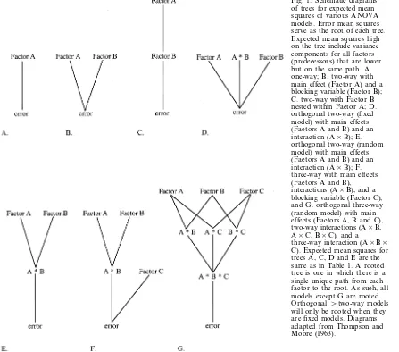
Fig. 1. Schematic diagrams of trees for expected mean squares of various ANOVA models. Error mean squares serve as the root of each tree. Expected mean squares high on the tree include variance components for all factors (predecessors) that are lower but on the same path. A. one-way; B. two-way with main effect (Factor A) and a blocking variable (Factor B); C. two-way with Factor B nested within Factor A; D. orthogonal two-way (fixed model) with main effects (Factors A and B) and an interaction (A×B); E. orthogonal two-way (random model) with main effects (Factors A and B) and an interaction (A×B); F. three-way with main effects (Factors A and B), interactions (A×B), and a blocking variable (Factor C); and G. orthogonal three-way (random model) with main effects (Factors A, B and C), two-way interactions (A×B, A×C, B×C), and a
three-way interaction (A×B× C). Expected mean squares for trees A, C, D and E are the same as in Table 1. A rooted tree is one in which there is a single unique path from each factor to the root. As such, all models except G are rooted. Orthogonal \two-way models will only be rooted when they are fixed models. Diagrams adapted from Thompson and Moore (1963).
two-way, and simple blocked and nested designs)
whereas others (orthogonal \two-way designs) can
not. If the ANOVA model in question can not be described by a rooted tree, then the ‘‘pool-the-mini-mum-violator’’ algorithm cannot be used and the re-searcher must resort to one of the other remediation procedures described above; limitation of magnitude of effects estimates to only significant factors will likely be the most useful option. If a tree is found to be rooted, the next step is to determine whether a minimum violator is present. A minimum violator is a point whose mean square is lower than that of its predecessor (Table 2, step 1). If a minimum violator is present then the sums of squares and degrees of freedom of the violator are combined with that of its predecessor and a pooled mean square is determined (Table 2, step 2). A new rooted tree is then created and additional mini-mum violators identified. The procedure continues until violators are no longer present in the tree. In a final
step, the pooled mean square is equated to each of the factors that comprise it, and variance components and magnitude of effects are determined based on these pooled estimates (Table 2, step 2). Such a procedure will result in unbiased variance component estimates for a wide variety of ANOVA models (Thompson and Moore 1963).
Use of magnitude of effects in ecology
response variable may not otherwise be clear. For
example, individual factors in a multi-factorial
ANOVA may be highly significant and the interactions among these factors may also be highly significant; 96 of 129 multi-factorial ANOVAs published in Australian Journal of Ecology, Ecology, Journal of Ecology, and Oikos published in 1998 detected significant higher-or-der interactions. In such cases, the effects of the individ-ual factors are not additive and proper analyses should only proceed by investigating the interaction terms in further detail. Underwood (1981, 1997) gave excellent discussions of the meaning of main effects in the pres-ence of interactions. Yet, when factors are not additive,
P values alone provide little information to the
re-searcher as to the relative importance of the main effects vs that of their interactions. Such relative com-parisons will clearly be of benefit during data analysis and interpretation. For instance, most of the variance in a response variable might be explained by the inter-action term, and thus a researcher who stresses the importance of main effects would clearly be drawing inappropriate conclusions. In contrast, a significant in-teraction term that has only weak effects on a response variable might suggest that, although not statistically
additive, it is the main effects that are of greater relative importance to the response variable.
We have found that estimating magnitude of effects is particularly informative when done in association with nested analyses, especially those that compare variability among various spatial or temporal scales (Graham 1999, M. S. Edwards unpubl.). In such de-signs, geographic areas or temporal periods can be partitioned into increasingly smaller units (scales). Each scale is nested within (and subsequently the level of
replication for) the next larger scale (Underwood 1997). A fully nestedn-factor ANOVA (n=number of scales) can then be used to determine at which spatial or temporal scale(s) variation in the response variable is significant, while estimating magnitude of effects can be used to compare relative variability among the scales. However, as discussed earlier, there is an increased likelihood of obtaining negative estimates of magnitude of effects in such models. These can occur when re-sponse variables are strongly regulated by variability at small spatial or temporal scales, and where variation at larger scales is reduced due to averaging of small-scale variability (Wiens 1989). In such cases, variability at the larger scales will be inherently less than at smaller scales, and the subsequent rearrangement and isolation of expected mean squares may result in negative vari-ance components estimates for some of the larger scales (see Table 1). The ‘‘pool-the-minimum-violator’’ tech-nique is a useful remedy when such cases occur (Gra-ham 1999, M. S. Edwards unpubl.).
We have come across a dozen or so ecological studies that have successfully used variance components and magnitude of effects to determine either the relative importance of individual factors and higher-order inter-actions (Forrester 1994, Levin et al. 1997, Price and Joyner 1997, Coomes and Grubb 1998, Rank et al. 1998, Casselle 1999, Lotze et al. 1999, Menge et al. 1999) or the spatio-temporal scales at which response variables are both significant and ‘most variable’ (Caf-fey 1985, Lively et al. 1993, Connell et al. 1997, Dun-stan and Johnson 1998, Graham 1999, Hughes et al. 1999). Of these, a compelling example of the benefits of estimating factor fit comes from Dunstan and John-son’s (1998) study of spatio-temporal variability in
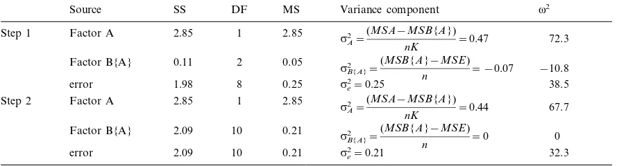
Table 2. Demonstration of the ‘‘pool-the-minimum-violator’’ technique for remediating negative variance components during determination of magnitude of effects in ANOVA. Data, model, and symbols were the same as in the nested example in Table 1. The model formed a rooted tree (Fig. 1C) with Factor B having a negative variance component and an unreasonable magnitude of effects estimate (Step 1). Factor B’s mean square was lower than that of its predecessor (the error mean square), identifying Factor B as the minimum violator in this model (Step 1). Sums of squares and degrees of freedom for the minimum violator and its predecessor were combined resulting in the calculation of a pooled mean square for the two sources (Step 2). Variance components were then recalculated for each source based on the pooled mean square, subsequently setting the variance component for Factor B to zero (Step 2); no minimum violators remained in the model. Magnitude of effects were then determined by dividing the new variance components for each factor by the sum of all variance components for the model (i.e. 0.65). In this example, Factor A explained 67.7% of variance in the response variable, Factor B explained 0%, and sampling error accounted for 32.3%.
Source SS DF MS Variance component v2
2.85 1
2.85 Factor A
Step 1 72.3
sA2=
(MSA−MSB{A})
nK =0.47
Factor B{A} 0.11 2 0.05 −10.8
sB2{A}=
(MSB{A}−MSE)
n = −0.07
error 1.98 8 0.25 se2=0.25 38.5
Factor A
Step 2 2.85 1 2.85
sA2=
(MSA−MSB{A})
nK =0.44 67.7
0.21
Factor B{A} 2.09 10
sB2{A}=
(MSB{A}−MSE)
n =0 0
10 0.21 se2=0.21 32.3
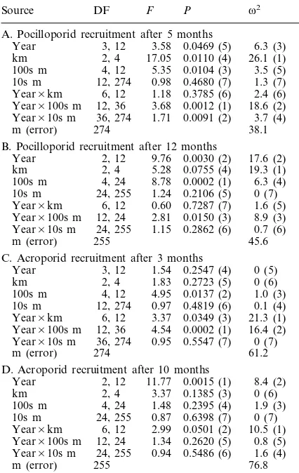
Table 3. ANOVA results from Dunstan and Johnson’s (1998) study of spatio-temporal variability in coral recruitment. All data are as presented in Dunstan and Johnson (1998). Origi-nal sources Zone, Sites {Zone}, Racks {Sites}, and error have been renamed km, 100s m, 10s m, and m, respectively. Paren-theses indicate rankings of significance (P) and magnitude of effects (v2) values within each experiment (A–D).
Source DF F P v2
A. Pocilloporid recruitment after 5 months
Year 3, 12 3.58 0.0469 (5) 6.3 (3) km 2, 4 17.05 0.0110 (4) 26.1 (1) 3.5 (5) 100s m 4, 12 5.35 0.0104 (3)
10s m 12, 274 0.98 0.4680 (7) 1.3 (7) Year×km 6, 12 1.18 0.3785 (6) 2.4 (6) Year×100s m 12, 36 3.68 0.0012 (1) 18.6 (2) Year×10s m 36, 274 1.71 0.0091 (2) 3.7 (4)
m (error) 274 38.1
B. Pocilloporid recruitment after 12 months
Year 2, 12 9.76 0.0030 (2) 17.6 (2) km 2, 4 5.28 0.0755 (4) 19.3 (1) 100s m 4, 24 8.78 0.0002 (1) 6.3 (4) 10s m 24, 255 1.24 0.2106 (5) 0 (7) Year×km 6, 12 0.60 0.7287 (7) 1.6 (5) Year×100s m 12, 24 2.81 0.0150 (3) 8.9 (3) Year×10s m 24, 255 1.15 0.2862 (6) 0.7 (6)
45.6 m (error) 255
C. Acroporid recruitment after 3 months
0 (5) Year 3, 12 1.54 0.2547 (4)
km 2, 4 1.83 0.2723 (5) 0 (6)
100s m 4, 12 4.95 0.0137 (2) 1.0 (3) 10s m 12, 274 0.97 0.4819 (6) 0.1 (4) Year×km 6, 12 3.37 0.0349 (3) 21.3 (1) Year×100s m 12, 36 4.54 0.0002 (1) 16.4 (2) Year×10s m 36, 274 0.95 0.5547 (7) 0 (7)
m (error) 274 61.2
D. Acroporid recruitment after 10 months
Year 2, 12 11.77 0.0015 (1) 8.4 (2) 0 (6)
km 2, 4 3.37 0.1385 (3)
100s m 4, 24 1.48 0.2395 (4) 1.9 (3) 10s m 24, 255 0.87 0.6398 (7) 0 (7) Year×km 6, 12 2.99 0.0501 (2) 10.5 (1) Year×100s m 12, 24 1.34 0.2620 (5) 0.8 (5) Year×10s m 24, 255 0.94 0.5486 (6) 1.6 (4)
m (error) 255 76.8
the variability in recruitment of pocilloporids and 60 – 80% of acroporids occurred at the scale of meters. Second, the results of Dunstan and Johnson (1998) clearly indicated that important patterns in ecological data can remain hidden if described by significance values alone. In each of four ANOVAs, the most significant main effect or interaction term did not have the greatest fit (Table 3), and in one case (Table 3B) the most significant term (100s m) explained less than 1/3 of the variance explained by an insignificant term (km). Furthermore, some interactions were highly significant and had high magnitude of effects (e.g. Year×100s m; Table 3A, C), whereas other interactions were either highly significant and had low magnitude of effects (Year×10s m; Table 3A) or weakly significant and had
high magnitude of effects (Year×km; Table 3C, D).
Consequently, although the most insignificant terms did have the lowest magnitude of effects, analysis of signifi-cance values alone would have generated misleading patterns of the relative importance of individual factors.
Ecologists rarely include estimates of factor fit in the description of ANOVA results, despite the widespread use of multi-factorial ANOVA in ecology. Yet, the logic and methodology presented here for determining magnitude of effects is quite intuitive and can be ap-plied to almost any ANOVA model for which expected mean squares can be determined for the individual factors. We have shown that estimates of factor fit can greatly enhance the analysis and interpretation of eco-logical ANOVAs, and we hope that ecologists will use the techniques described herein with the goal that they become incorporated into the conventional routine for analyzing ecological data with ANOVA.
Acknowledgements – We thank P. Raimondi for statistical advice, L. Ferry-Graham for encouragement, and J. Estes, P. Raimondi, G. Leonard, E. Sala, and A. Stewart-Oaten for reviewing early versions of the manuscript. MHG was sup-ported during manuscript preparation by a grant from the NOAA/National Sea Grant (cNA66RG0477) and California Sea Grant (cR/CZ-141) programs, and MSE was supported by a grant from the National Science Foundation (OCE-9813562).
References
Bennington, C. C. and Thayne, W. V. 1994. Use and misuse of mixed model analysis of variance in ecological studies. – Ecology 75: 717 – 722.
Berlow, E. L. 1999. Strong effect of weak interactions in ecological communities. – Nature 398: 330 – 334. Burdick, R. K. and Graybill, F. A. 1992. Confidence intervals
on variance components. – M. Dekker.
Caffey, H. M. 1985. Spatial and temporal variation in settle-ment and recruitsettle-ment of intertidal barnacles. – Ecol. Monogr. 55: 313 – 332.
Casselle, J. E. 1999. Early post-settlement mortality in a coral reef fish and its effects on local population size. – Ecol. Monogr. 69: 177 – 194.
Connell, J. H., Hughes, T. P. and Wallace, C. C. 1997. A 30-year study of coral abundance, recruitment, and distur-bance at several scales in space and time. – Ecol. Monogr. 67: 461 – 488.
Coomes, D. A. and Grubb, P. J. 1998. Responses of juvenile trees to above- and belowground competition in nutrient-starved Amazonian rain forest. – Ecology 79: 768 – 782. Dodd, D. H. and Schultz, R. F. Jr. 1973.
Computa-tional procedures for estimating magnitude of effect for some analysis of variance designs. – Psychol. Bull. 79: 391 – 395.
Dunstan, P. K. and Johnson, C. R. 1998. Spatio-temporal variation in coral recruitment at different scales on Heron Reef, southern Great Barrier Reef. – Coral Reefs 17: 71 – 81.
Forrester, G. E. 1994. Influences of predatory fish on density and dispersal of stream insects. – Ecology 75: 1208 – 1218. Graham, M. H. 1999. Identification of kelp zoospores from in
situ plankton samples. – Mar. Biol. 135: 709 – 720. Hughes, T. P., Baird, A. H., Dinsdale, E. A. et al. 1999.
Patterns of recruitment and abundance of corals along the Great Barrier reef. – Nature 397: 59 – 63.
Karlson, R. H. and Cornell, H. V. 1998. Scale-dependent variation in local vs. regional effects on coral species richness. – Ecol. Monogr. 68: 259 – 274.
Kingsford, M. and Battershill, C. 1998. Studying temperate marine environments: a handbook for ecologists. – Canter-bury Univ. Press.
Levin, P. S., Chiasson, W. and Green, J. M. 1997. Geographic differences in recruitment and population structure of a temperate reef fish. – Mar. Ecol. Prog. Ser. 161: 23 – 35. Lively, C. M., Raimondi, P. T. and Delph, L. F. 1993.
Intertidal community structure: space-time interactions in the northern Gulf of California. – Ecology 74: 162 – 173. Lotze, H. K., Schramm, W., Schories, D. and Worm, B. 1999.
Control of macroalgal blooms at early developmental stages:Pilayella littoralisversusEnteromorpha spp. – Oe-cologia 119: 46 – 54.
Menge, B. A., Daley, B. A., Lubchenco, J. et al. 1999. Top-down and bottom-up regulation of New Zealand rocky intertidal communities. – Ecol. Monogr. 69: 297 – 330.
Neter, J., Kutner, M. H., Nachtscheim, C. J. and Wasserman, W. 1996. Applied linear statistical models. – McGraw-Hill. Newman, J. A., Bergelson, J. and Grafen, A. 1997. Blocking
factors and hypothesis tests in ecology: is your statistics text wrong? – Ecology 78: 1312 – 1320.
Paine, R. T. 1992. Food-web analysis through field measure-ment of per capita interaction strength. – Nature 355: 73 – 75.
Potvin, C. 1993. Experiments in controlled environments. – In: Scheiner, S. M. and Gurevitch, J. (eds), Design and analysis of ecological experiments. Chapman and Hall, pp. 46 – 68.
Price, M. V. and Joyner, J. W. 1997. What resources are available to desert granivores: seed rain or soil seed bank? – Ecology 78: 764 – 773.
Rank, N. E., Kopf, A., Julkunen-Tiitto, R. and Tahvanainen, J. 1998. Host performance of the salicylate-using beetle
Phratora6itellinae. – Ecology 79: 618 – 631.
Searle, S. R., Casella, G. and McCulloch, C. E. 1992. Variance components. – J. Wiley and Sons.
Sokal, R. R. and Rohlf, F. J. 1981. Biometry. – W. H. Freeman.
Thompson, W. A. Jr. 1962. The problem of negative estimates of variance components. – Ann. Math. Stat. 33: 273 – 289. Thompson, W. A. Jr. and Moore, J. R. 1963. Non-negative estimates of variance components. – Technometrics 5: 441 – 449.
Underwood, A. J. 1981. Techniques of analysis of variance in experimental marine biology and ecology. – Oceanogr. Mar. Biol. Annu. Rev. 19: 513 – 605.
Underwood, A. J. 1997. Experiments in ecology. – Cambridge Univ. Press.
Underwood, A. J. and Petraitis, P. S. 1993. Structure of intertidal assemblages in different locations: how can local processes be compared? – In: Ricklefs, R. E. and Schluter, D. (eds), Species diversity in ecological communities. Univ. of Chicago Press, pp. 39 – 51.
Vaughn, G. M. and Corballis, M. C. 1969. Beyond tests of significance: estimating strength of effect in selected ANOVA designs. – Psychol. Bull. 72: 204 – 213.
Weldon, C. W. and Slauson, W. L. 1986. The intensity of competition versus its importance: an overlooked distinc-tion and some implicadistinc-tions. – Q. Rev. Biol. 61: 23 – 43. Wiens, J. A. 1989. Spatial scaling in ecology. – Funct. Ecol. 3:
385 – 398.
Winer, B. J., Brown, D. R. and Michels, K. M. 1991. Statisti-cal principles in experimental design. – McGraw-Hill. Zar, J. H. 1996. Biostatistical analysis. – Prentice-Hall.