Full Terms & Conditions of access and use can be found at
http://www.tandfonline.com/action/journalInformation?journalCode=ubes20
Download by: [Universitas Maritim Raja Ali Haji] Date: 13 January 2016, At: 00:38
Journal of Business & Economic Statistics
ISSN: 0735-0015 (Print) 1537-2707 (Online) Journal homepage: http://www.tandfonline.com/loi/ubes20
A Note on Rubin's Statistical Matching Using
File Concatenation With Adjusted Weights and
Multiple Imputations
Chris Moriarity & Fritz Scheuren
To cite this article: Chris Moriarity & Fritz Scheuren (2003) A Note on Rubin's Statistical
Matching Using File Concatenation With Adjusted Weights and Multiple Imputations, Journal of Business & Economic Statistics, 21:1, 65-73, DOI: 10.1198/073500102288618766
To link to this article: http://dx.doi.org/10.1198/073500102288618766
Published online: 01 Jan 2012.
Submit your article to this journal
Article views: 74
View related articles
A Note on Rubin’s Statistical Matching Using
File Concatenation With Adjusted Weights
and Multiple Imputations
Chris
Moriarity
U.S. General Accounting Of’ce (chrismor@cpcug.org)
Fritz
Scheuren
NORC, University of Chicago (scheuren@aol.com)
Statistical matching has been used for more than 30 years to combine information contained in two sample survey les. Rubin (1986) outlined an imputation procedure for statistical matching that is different from almost all other work on this topic. Here we evaluate and extend Rubin’s procedure.
KEY WORDS: Complex survey design; Multivariate normal; Predictive mean matching; Resampling; Robustness; Variance-covariance structures.
1. INTRODUCTION
Statistical matching began to be widely practiced with the availability of public use les in the 1960s (Citro and Hanushek 1991). Arguably, the desire to use this technique was even an impetus for the release of several early public use les, including those involving U.S. tax and census data (e.g., Okner 1972).
Statistical matching continues to be widely used by economists for policy microsimulation modeling in govern-ment, its original home (as the references herein attest). It also has begun to play a role in many business settings as well, especially as a way—in an era of data warehousing and data mining—to bridge across information silos in large orga-nizations. These applications have not yet reached refereed journals, however—partly, we believe, because they are being treated as proprietary.
Despite their widespread and, in some areas, growing use, statistical matching techniques seem to have received insuf-cient attention regarding their theoretical properties. Statistical matching always has had an ad hoc avor (Scheuren 1989), although parts of the subject have been examined with care (e.g., Cohen 1991; Rodgers 1984; Sims 1972). In this article we return to one of the important attempts to underpin prac-tice with theory, important work of Don Rubin (1986), now more than 15 years old.
We begin by describing Rubin’s contribution. Needed renements are then made that go hand-in-hand with advances in computing in the time since Rubin’s article was written. To frame the results presented, after this introduction (Sec. 1) we include a section (Sec. 2) titled “What is Statistical Match-ing?” This is followed by a restatement of Rubin’s original results, along with a detailed examination of the method’s properties (Sec. 3). Then in Section 4 we present improve-ments of Rubin’s procedure and develop their properties. In Section 5 we provide some simulation results that illustrate the new approaches, and in Section 6 discuss applications and generalizations of the approaches. Finally, in Section 7 we give a summary and draw some conclusions.
2. WHAT IS STATISTICAL MATCHING?
Perhaps the best description to date of statistical match-ing has been given by Rodgers (1984); other good descrip-tions have been given by Cohen (1991) and Radner, Allen, Gonzalez, Jabine, and Muller (1980). A brief summary of the method is provided here.
Suppose that there are two sample les, A and B, taken from two different surveys. Suppose further that le A con-tains potentially vector-valued variables4X1 Y 5, whereas le B contains potentially vector-valued variables4X1 Z5. The objec-tive of statistical matching is to combine these two les to obtain at least one le containing 4X1 Y 1 Z5. In contrast to
record linkage, or exact matching (e.g., Fellegi and Sunter 1969; Scheuren and Winkler 1993, 1997), the two les to be combined are notassumed to have records for the same enti-ties. In statistical matching, the les are assumed to have little or no overlap, and hence records forsimilarentities are com-bined, rather than records for thesame entities.
All statistical matches described in the literature have used the X variables in the two les as a bridge to create synthetic records containing4X1 Y 1 Z5. To illustrate, suppose that le A consisted in part of records
X11 Y11 X21 Y21
and
X31 Y31 whereas le B had records of the form
X11 Z11
X31 Z31
©2003 American Statistical Association Journal of Business & Economic Statistics January 2003, Vol. 21, No. 1 DOI 10.1198/073500102288618766
65
66 Journal of Business & Economic Statistics, January 2003
and
X41 Z40
The matching methodologies used almost always have made the assumption that 4Y 1 Z5 are conditionally independent given X, as pointed out initially by Sims (1972). From this assumption, it would be immediate that one could create
X11 Y11 Z1 and
X31 Y31 Z30
Notice that matching on X1 and X3 in no way implies that [4X11 Y15and4X11 Z15], or [4X31 Y35and 4X31 Z35], are taken from the same entities.
What to do with the remaining records is less clear, and techniques vary. Broadly, the various strategies used for sta-tistical matching can be grouped into two general cate-gories, “constrained” and “unconstrained.” Constrained statis-tical matching requires the use of all records in the two les and basically preserves the marginal Y and Z distributions (e.g., Barr, Stewart, and Turner 1982). In the foregoing (sim-plistic) example, for a constrained match one would have to end up with a combined le that also had records
X21 Y21 Z?? and
X41 Y??1 Z40
Unconstrained matching does not have this requirement, and one might stop after creating X21 Y21 Z??. How the statistical matching procedure dened records to besimilarwould deter-mine the values of the variables without specic subscripts.
A number of practical issues, not part of our present scope, need to be addressed during a statistical matching process. Among these issues are alignment of universes (i.e., agree-ment of the weighted sums of the data les) and alignagree-ment of units of analysis (i.e., individual records representing the same units). Usually, too, the bridgingX variables can have different measurement or nonsampling properties in the two les (See Cohen 1991; Ingram, O’Hare, Scheuren, and Turek 2000 for further details).
Statistical matching is by no means the only way to com-bine information from two les. Sims (1978), for instance, described alternative methodologies to statistical matching that could be used under conditional independence. Other authors (e.g., Singh, Mantel, Kinack, and Rowe 1993; Paass 1986, 1989) have described methodologies for statistical matching if auxiliary information about the4Y 1 Z5relationship is avail-able. Although an important special case, this option is seldom available (Ingram et al. 2000). (See also National Research Council 1992, where the subject of combining information has been taken up quite generally.)
Rodgers (1984) included a more detailed example of com-bining two les using both constrained and unconstrained matching than the example that we provide here. We encour-age the interested reader to consult that reference for an illustration of how sample weights are used in the matching process.
3. RUBIN’S PROCEDURE FOR STATISTICAL MATCHING
In the framework described earlier, Rubin (1986) outlined a methodology for what he termed the “concatenation” of two sample les. Assuming a trivariate outcome le 4X1 Y 1 Z5, whereXcould be vector-valued, Rubin suggested a methodol-ogy for multiple imputation (Rubin 1987, 1996) ofZin le A andY in le B, based on several specied values of the par-tial correlation ofY andZ, givenX. We rst describe Rubin’s procedure, and then examine aspects of the procedure in more detail.
3.1 Description of the Procedure
Broadly, Rubin proposes starting his procedure by using regression. This in turn creates the predictions of the variables that he wants to use for the statistical matching. Finally, he advocates concatenating the resulting les.
Each of these steps is described briey in this section, fol-lowed by a discussion in Section 3.2 of the procedure’s the-oretical properties. As will be seen, many of these thethe-oretical results are new and in places corrective. In fact, we would not advocate using Rubin’s approach without major modications, as we specify in Sections 4 and 6.
3.1.1. Regression Step. Rubin’s procedure begins by postulating a value for the partial correlation of4Y 1 Z5 given
X, and calculating the regressions ofY on X in le A andZ
on X in le B. The regression coefcients, the variances of the residuals from the two regressions, and the assumed value of the partial correlation of4Y 1 Z5, givenX, then are used to construct the matrix
0 B @
0 RYonX RZonX
ƒ4RYonX50 pvarY—X pcovY 1 Z—X
ƒ4RZonX50 pcovY 1 Z—X pvarZ—X
1 C
A0 (1)
Here RYonX andRZonX are the column vectors of the
regres-sion coefcients of Y on X and Z on X, respectively, and ƒ4RYonX5
0 and ƒ4R
ZonX5
0 are the respective negative
trans-poses.RYonXandRZonX are of dimension4mC15by 1, where
the dimension of X is m. pcovY 1 Z—X is the partial covariance
of4Y 1 Z5 givenX; pvarY—X is the partial variance of Y given
X, and pvarZ—X is the partial variance of Z given X. pvarY—X
and pvarZ—X are estimated using the variances of the residuals
of the corresponding regressions, and pcovY 1 Z—X is estimated
using the assumed value of the partial correlation of 4Y 1 Z5, givenX, multiplied by the square root of (pvarY—X¢pvarZ—X).
The “sweep” matrix operator (Goodnight 1979; Seber 1977) is then applied to (1) to obtain estimates of RYonX1 Z and
RZonX1 Y. Beginning with (1) and then “sweeping onY” gives
the matrix
0 B @
# # 4RZonX 1 Y512nƒ1 # # 4RZonX 1 Y5n
ƒ4RZonX1 Y5012nƒ1 ƒ4RZonX1 Y5n pvarZ—X1 Y
1 C A1
and beginning with (1) and “sweeping onZ” gives the matrix
denotes the full set of regression coefcients of A on B and C.
RYonX1 Z is used to obtain what we call the “primary”
esti-mates of Y in le B, andRZonX1 Y is used to obtain primary
estimates ofZin leA. These primary predicted values then are used to produce what we call the “secondary” predicted values.RYonX1 Z is used, along with observedX and predicted
Z, to obtain secondary estimates ofY in le A, andRZonX 1 Y
is used, along with observedX and predictedY, to obtain sec-ondary estimates ofZin le B.
At the completion of the estimation step, le A consists of observedX, observedY, primary predictedZ, and secondary predictedY. File B consists of observedX, observed Z, pri-mary predictedY, and secondary predictedZ.
Note that if the partial correlation of Y andZ, givenX, is assumed to be 0, then the foregoing procedure simplies. In this case,RYonX1 Z equalsRYonX andRZonX1 Y equalsRZonX.
We note in passing that the regression coefcients obtained by use of the sweep operator as described by Rubin also can be obtained by the regression method described by Kadane (1978). (See Goodnight 1979 or Seber 1977, chap. 12 for more details.) The methods are identical if applied to just one dataset, and differences in regression coefcients obtained from the two methods in the framework discussed here can be expected to be small if the datasets are large.
To replicate the regression coefcients shown in Rubin’s table 5, we need to use the sweep operator, because the datasets are very small (eight records in le A and six records in le B). However, even in this case, Kadane’s method pro-duces regression coefcients ofY onX andZin good ment with Rubin’s method. (Note, however, that the agree-ment is not too good for the regression coefcients ofZonX
andY.)
3.1.2. Matching Step. The matching step in Rubin’s approach involves using unconstrained matches. The nal value ofZassigned to thejth record in le A is obtained by doing an unconstrained match between the (primary) predicted value of Z for the jth record and the (secondary) predicted values ofZ in le B. (The matching criterion is a minimum distance or nearest-neighbor approach.) The observedZvalue in the matched record in le B is then assigned to the jth record in le A. Similarly, the nal value of Y assigned to theith record in le B is obtained by doing an unconstrained match between the (primary) predicted value ofY for theith record and the (secondary) predicted values of Y in le A. The matching steps are done separately forY andZ.
Note that a careful reading of Rubin’s article is necessary to discern his methodology for the matching step. The sta-tistical matching literature contains references that incorrectly state that Rubin’s procedure is to do an unconstrained match between the (primary) predicted value ofZfor thejth record in le A and theobservedvalues ofZin le B, and an uncon-strained match between the (primary) predicted value ofY for theith record in le B and theobservedvalues ofY in le A.
3.1.3. Concatenation Step. Rubin then suggests concate-nating the resulting statistically matched les and assigning the weight 4wƒ1 weight corresponding to the le A portion of the record and wB is the weight corresponding to the le B portion of the record.
Rubin’s method is one of only two procedures described in the statistical matching literature for assessing the effect of alternative assumptions of the inestimable value cov4Y 1 Z5. (See Kadane 1978, supplemented by Moriarity 2001, for the other procedure.)
Rubin suggests that his basic procedure be repeated for sev-eral assumed values of the partial correlation of4Y 1 Z5 given
X, as an operation akin to multiple imputation (Rubin 1987, 1996). Note that Kadane (1978) had already emphasized the necessity of repeating the matching procedure for a range of corr4Y 1 Z5 values, thus anticipating Rubin’s multiple imputa-tion concept as applied in this arena.
3.2 Further Aspects of Rubin’s Method
Here we discuss some aspects of Rubin’s method separately for the regression step, matching step, and concatenation step.
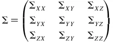
3.2.1. Regression Step. In this section we discuss Rubin’s method within the framework of 4X1 Y 1 Z5 hav-ing a nonshav-ingular multivariate normal distribution with mean
4ŒX1 ŒY1 ŒZ5and covariance matrix
All elements ofècan be estimated from le A or le B except forèY Z and its transpose,èZY. Specication of the partial
cor-relation of4Y 1 Z5givenX, as Rubin does, can be considered equivalent to specication ofèY Z in this framework.
It can be shown (Moriarity 2001) that for le A, after the “primary” prediction ofZ, the joint distribution of4Xj1 Yj1bZj5
We use the “A1” subscript to emphasize that this is the covari-ance matrix for le A, after the primary prediction ofZ.èZbZb
can be shown to equal
¡
Similarly, it can be shown that for le B, after the primary prediction ofY, the joint distribution of4Xi1bYi1 Zi5 in le B
68 Journal of Business & Economic Statistics, January 2003
Hence, although the variances of the variables created by pre-diction are smaller than the variances of the variables being predicted (see Sec. 4 for more discussion of this assertion), other relationships are preserved. In particular, the postulated value ofèY Z is preserved.
In le A, after the “secondary” prediction of Y, it can be shown (Moriarity 2001) that the joint distribution of
4Xj1eYj1bZj5 is normal with mean 4ŒX1 ŒY1 ŒZ5 and singular
Similarly, in le B, after the secondary prediction ofZ, it can be shown that the joint distribution of4Xi1bYi1eZi5 is
nor-3.2.2. Matching Step. Rubin’s procedure uses uncon-strained matching. This allows for the possibility that some records in each le act as a “donor” more than once, whereas other records are not used. Unlike constrained matching, which forces the use of all records, unconstrained matching can lead to distortions in means, variances, and other param-eters (see, e.g., Rodgers 1984).
3.2.3. Concatenation Step. As mentioned earlier, Rubin suggests concatenating the les and assigning the weight
4wƒ1 A Cw
ƒ1 B 5
ƒ1to each record. If a given record consists mostly of data from le A, then wAis the weight corresponding to the le A portion of the record, and wB is the weight correspond-ing to the le B portion of the record under the assumption that it was sampled according to the protocol used to sample le A. If the given record consists mostly of data from le B, then wB is the weight corresponding to the le B portion of the record and wA is the weight corresponding to the le A portion of the record under the assumption that it was sampled according to the protocol used to sample le B.
This suggested weight is intuitively reasonable and feasible to compute in simple cases such as iid sampling. For iid sam-pling, it can be shown (as Rubin does) that estimates are unbi-ased. However, for more complex sampling designs, it may not be feasible to compute the suggested weight. The needed sam-ple design information may not be available, and/or it could be difcult or impossible to compute selection probabilities for records in one le under the assumption of sampling accord-ing to the protocol used to sample the other le.
A serious problem with concatenation after the use of unconstrained matching is that estimates may not be unbiased, given the use of unconstrained matching, for non-iid sampling. Furthermore, concatenation can give the illusion of the cre-ation of additional informcre-ation. If le A and le B have 200 records each, it seems apparent that it is not possible to form more than 200 matchedY-Zpairs; however, concatenation can give the illusion of up to 400Y-Z pairs. This problem of the illusion of having more information is a criticism that can, of course, in one way or another be leveled at all statistical matching methods.
4. LOSS OF SPECIFIED VALUE OFèY Z IN RUBIN’S PROCEDURE: ALTERNATIVES CONSIDERED
In the ideal situation of statistically matching two data les, each having many observations with variables that are multi-variate normally distributed, the preferred outcome of a pro-cedure such as Rubin’s would be that a specied value ofèY Z
is reproduced accurately in the nal product of the statistical matching procedure. Other characteristics such as means, vari-ances, and covariances that are observable in les A and B should also be preserved.
For Rubin’s procedure, the results presented in Section 3.2.1 show that the specied value of èY Z is preserved during the primary estimation of Y and Z in the multivariate normal framework. However, the specied value is not guaranteed to be preserved during the secondary estimation of Y andZ. In fact, signicant deviation is possible.
Our extensive simulation of Rubin’s suggested match-ing procedure (see Sec. 5 for details of the simulation
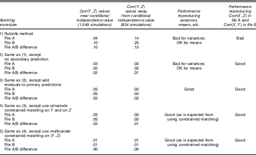
Table 1. Summary of Simulation Results for Rubin’s Method and Related Methods
Corr(Y1Z) Performance
Corr(Y1Z)values values away Performance reproducing near conditional from conditional reproducing Corr(X1Z)in Matching independence value independence value variances, ’le A and procedure (1,049 simulations) (824 simulations) means, etc. Corr(X1Y)in ’le B
(1) Rubin’s method
File A .04 .14 Bad for variances; Bad
File B .10 .25 OK for means
File A/B difference .10 .13
(2) Same as (1), except no secondary prediction
File A .03 .03 Bad for variances; Good
File B .02 .02 OK for means
File A/B difference .02 .01
(3) Same as (2), except add residuals to primary predictions
File A .03 .03 Good Good
File B .05 .03
File A/B difference .03 .02
(4) Same as (3), except use univariate constrained matching onYand onZ
File A .03 .03 Good (as is expected from Good
File B .05 .03 using constrained matching)
File A/B difference .03 .01
(5) Same as (4), except use multivariate constrained matching on(Y1Z)
File A .01 .01 Good (as is expected from Good
File B .01 .01 using constrained matching)
File A/B difference .00 .00
NOTE: The ’le A and ’le B rows show the average absolute differences between estimated Corr(Y1Z)and speci’ed Corr(Y1Z). The ’le A/B difference row shows the average absolute difference between estimates of Corr(Y1Z)in the two ’les.
methodology) showed that the specied value of èY Z is not
always preserved in the nal les. Not surprisingly, there was considerable correlation between the divergence of the esti-mated value of èY Z from the specied value of èY Z and the
divergence of èbYeZ from èY Z. Furthermore, the estimates of
èY Zcomputed from the two les often were far apart—a
trou-bling inconsistency. Hence, Rubin’s methodology needed to be revised to address these anomalies.
One alternative possibility is to carry out a modication of Rubin’s procedure in which the secondary estimation step is omitted, to eliminate the distortions introduced by that step. That is, an alternative procedure is to use actual values, rather than secondary estimates, during the matching step. As shown in Table 1, our simulations provided strong evidence that this modication of Rubin’s procedure was far more successful on average in retaining the specied value ofèY Z. This modi-cation also attained much better consistency of the estimated values ofèY Z from the two les compared with Rubin’s pro-cedure.
A second alternative possibility to consider is to impute residuals to the primary predicted values before the matching step. Note that èZZƒèbZbZ and èY YƒèbYbY can be identied
as variances of random variables with certainconditional dis-tributions(e.g., Anderson 1984, p. 37). (This also shows that the variances of the predicted variable values are smaller than the variances of the variables themselves.) Hence the covari-ance matrices can be made equal by imputing independently drawn normally distributed random residuals with mean 0 and
variance as specied and adding these residuals toZbj andbYi.
As shown in Table 1, simulations suggest that this methodol-ogy is comparable in most ways to Rubin’s procedure with-out the secondary estimation step. However, this methodology provided improved performance in reproducing variances.
A third alternative methodology is to proceed as in the aforementioned alternative, except to replace unconstrained matching onY and onZwith univariateconstrained matching
onY and onZ(two separate matches). As shown in Table 1, the results of this alternative are comparable to those of the two previous alternatives. However, this procedure has the additional benet of guaranteeing the elimination of distortion in variances that can occur when unconstrained matching is used.
A fourth alternative to consider is to proceed as in the foregoing alternative, but replace two univariate constrained matches onY and onZwith a singlemultivariateconstrained match on4Y 1 Z5. This alternative, which consists of the pri-mary estimation step, skipping the secondary estimation step, and multivariate constrained matching on 4Y 1 Z5 after impu-tation of residuals, has been discussed at length by Moriarity (2001) and Moriarity and Scheuren (2001). The multivariate constrained matching step uses a Mahalanobis distance com-puted on4Y 1 Z5and was implemented in our simulations using the RELAX-IV public domain software (Bertsekas 1991; Bert-sekas and Tseng 1994). If the matching step links the jth record in le A to theith record of le B, then the nal value ofZ assigned to thejth record in le A comes from theith
70 Journal of Business & Economic Statistics, January 2003
record of le B, and the nal value of Y assigned to the ith record of File B comes from thejth record of File A.
This fourth alternative has the benets of univariate con-strained matching, and it also eliminates any inconsistency between 4Y 1 Z5 estimates using le A and 4Y 1 Z5 estimates using le B. As shown in Table 1, this alternative gave the best performance of the methods considered.
5. DESCRIPTION AND RESULTS OF THE SIMULATION METHODOLOGY
To assess the performance of Rubin’s procedure, and vari-ants of that procedure, we carried out simulations. In these simulations we used univariateX, Y, andZ, with 4X1 Y 1 Z5
assumed to have a trivariate normal distribution. Without loss of generality, 4X1 Y 1 Z5 were assumed to have zero means and unit variances. In this simple framework,èY Z is equal to Corr4Y 1 Z5, and so on.
Corr4X1 Y 5 was allowed to vary from 0 to .95 in incre-ments of .05. For a given value of Corr4X1 Y 5, Corr4X1 Z5
was allowed to vary from Corr4X1 Y 5to .95 in increments of .05. For given values of Corr4X1 Y 5 and Corr4X1 Z5 values, Corr4Y 1 Z5 was allowed to take a range of 4–10 different val-ues within the bounds specied by
Corr4X1 Y 5¢Corr4X1 Z5
p
61ƒ4Corr4X1 Y 5527
¢61ƒ4Corr4X1 Z55271
which can be estimated using le A and le B. These bounds have been variously derived (Rodgers and DeVol 1982; Moriarity 2001). All start with the requirement that the corre-lation matrix of4X1 Y 1 Z5must be positive denite.
Note that the number of values of Corr4Y 1 Z5depended on the length of the interval of admissible values of Corr4Y 1 Z5. For given values of Corr4X1 Y 5, Corr4X1 Z5, and Corr4Y 1 Z5, we drew two independent samples of size 1,000 from the specied multivariate normal distribution. We felt that using a sample size of 1,000 was a reasonable compromise to simulate a dataset of realistic size with minimal sampling variability, while avoiding excessive computational burden.
We carried out the regression steps as previously described in Section 3.1.1. Note that although it is possible to pool the
Xvalues from both les to estimate var4X5, this can and does lead to occasional problems of nonpositive denite covariance matrices (Moriarity 2001). To avoid such problems, we used
X values only from le A to estimate var4X5when predicting
ZfromX andY for le A, and usedX values only from le B to estimate var4X5when predictingY fromX andZfor le B. All of the simulation work, except for the fourth alternative discussed in the previous section, was carried out on a Pen-tium II PC with a 400 MHz processor and 128 MB of RAM. A set of about 2,000 simulations typically took several hours of continuous computer processing to complete. The simula-tion work for the fourth alternative was done separately (as discussed in Moriarity and Scheuren 2001), and required more computer processing (days, as compared to hours) than the other alternatives.
5.1 Results and Innovations
Table 1 summarizes the results of applying:
1. Rubin’s originally-proposed procedure and then the fol-lowing modications, as described in Section 4:
2. Skipping the use of secondary predicted values
3. Skipping the use of secondary predicted values and adding residuals to the primary predicted values before match-ing
4. Same as 3, except using univariate constrained match-ing onY and onZ (two separate matches) instead of uncon-strained matching onY and onZ
5. Same as 4, except using multivariate constrained match-ing on4Y 1 Z5.
Comparing the rst two columns within a given row reveals the relative performance of a matching procedure for values near conditional independence versus values far from con-ditional independence. For Rubin’s original method, perfor-mance was worse for values far from conditional indepen-dence. All of the modied procedures had robust performance relative to conditional independence.
Comparing the rows within one of the rst two columns illustrates the relative ability of different procedures to repro-duce the specied value of Corr4Y 1 Z5after the matching step. It can be seen that Rubin’s method had the poorest perfor-mance of all methods considered, due to the distortion intro-duced by the secondary estimation step. The best-performing procedure was the one that added residuals to primary predic-tions and then performed multivariate constrained matching using4Y 1 Z5.
As shown in Table 1, we performed a broader evaluation of the various procedures. We examined each procedure’s abil-ity to reproduce other estimates, such as E4Z5, var4Z5, and Corr4X1 Z5 in le A and E4Y 5, var4Y 5, and Corr4X1 Y 5 in le B. Overall, Rubin’s method again had the poorest compar-ative performance for reproducing variances and covariances. We think that this is because of the secondary estimation step, because methods that used unconstrained matching but not the secondary estimation step generally performed better. Overall, multivariate constrained matching had the best comparative performance for reproducing variances and covariances.
5.2 Simulation Summary
To summarize, we found that it was very important to eschew the secondary estimation step. Several procedures that omitted the secondary estimation step gave comparable results, with multivariate constrained matching performing the best.
6. APPLICATIONS AND GENERALIZATIONS
In this article we have made the assumption that the vari-ables to be statistically matched come from multivariate nor-mal distributions. This does not really t most situations in practice, where the variables come from complex survey designs and do not have a standard theoretical distribution, let alone a normal one.
In addition to problems that arise with Rubin’s method from carrying out secondary estimation, another limitation of the
method is that it assumes bivariate4Y 1 Z5. Generalizations to higher dimensions are not immediate. It may be possible to apply techniques akin tomultivariate predictive mean match-ing, as discussed by Little (1988). An alternative procedure that appears to generalize in a straightforward way to higher dimensions is discussed by Moriarity and Scheuren (2001).
Although developing a complete paradigm is beyond our scope here, we can make some suggestions:
1. Constrained matching is a good starting point. It is expensive but now affordable with recent advances in com-puting. The use of unconstrained matching by Rubin does not seem to be essential to his ideas; indeed, it may have been advocated just for the sake of specicity.
2. Applications that match les as large as 1,000 (the sam-ple size that we simulated) would be unusual. Even in large-scale projects, like matching the full Current Population Sur-vey with the SurSur-vey of Income and Program Participation, the matching generally would be done separately in modest-sized demographic subsets dened by categorical variables such as gender or race (e.g., as described in Ingram et al. 2000).
3. We believe that the general robustness of normal meth-ods can be appealed to, even when the individual observations are not normal. Although not necessarily optimal, the statistics calculated from the resulting combined le will be approxi-mately normal because of the central limit theorem.
4. Resampling of the original sample before using the tech-niques presented in this article, could help expose potential lack of robustness to failures in the iid assumption. One such technique was discussed by Hinkins, Oh, and Scheuren (1997). This can be computationally expensive, depending on the sam-ple designs of the two les being matched.
5. Often researchers who do statistical matching do not bring survey designers into the matching process. This is needed. The use of sample replication, even if only approxi-mately, is one way that designers can help matchers. Without help from samplers, it generally will not be possible to create credible sample variance estimates for statistics created from the matched les. This is formidable in any case but could be especially so with a concatenated le.
6. Deep subject matter knowledge is needed to deal with differences in the measurement error and other nonsampling concerns (e.g., edit and imputation issues) that arise and that may even be a dominant limitation to statistical matching.
7. In all applications, no matter what the matcher’s experi-ence level, caution would recommend that with a new prob-lem, simulations always be done and a small prototype involv-ing real data be conducted before beginninvolv-ing on a large scale. No decision on how (or even whether) to do a statistical match should be made until these steps have been taken.
7. SUMMARY AND CONCLUSIONS
Rubin’s 1986 article in the Journal of Business and Eco-nomic Statisticspresented innovative ideas in the area of sta-tistical matching that, although important, have not until now been followed up and developed. This is unfortunate, because the approach advocated by Rubin once modied, has value to practitioners.
7.1 Secondary Estimation
We have shown that Rubin’s procedure is sound during the primary estimation step, but not necessarily during the sec-ondary estimation step. In fact, we strongly advise against the routine use of Rubin’s secondary estimation step.
Because of the loss of the specied value ofèY Z that can
occur during the secondary estimation step, Rubin’s procedure is not feasible as originally described. However, innovations such as avoiding the secondary estimation step, adding resid-uals to the primary estimates before matching, and using con-strained matching, particularly multivariate concon-strained match-ing on4Y 1 Z5, appear to make the procedure feasible.
The end result is a collection of datasets formed from var-ious assumed values of èY Z, where analyses can be repeated
over the collection and the results can be averaged or summa-rized in some other meaningful way. (For a recent reference on ways to average the resulting values, see Hoeting, Madigan, Raftery, and Volinsky 1999). The methods described by Rubin (1987, 1996) also might be used; however, we consider this an area in which additional research is warranted.
7.2 Unconstrained Matching
Legitimate concerns also arise when unconstrained ing is used. The suggestion of using unconstrained match-ing was appealmatch-ing when made originally by Rubin, because it requires much less computational effort than multivariate constrained matching. However, it can be shown that uncon-strained matching leads to distortion of means and variances, as discussed by Rodgers (1984).
A simple form of univariate constrained matching (Goel and Ramalingam 1989) that matches ranked values is compa-rable in computational effort to unconstrained matching. This method appears to work acceptably when used in tandem with avoiding secondary estimation and adding residuals to the pri-mary estimates. Ingram et al. (2000) evaluated this procedure, but without residuals added. Multivariate constrained match-ing requires more computational effort, but advances in com-puter hardware and software (e.g., Bertsekas 1991; Bertsekas and Tseng 1994) have made multivariate constrained match-ing feasible.
7.3 Concatenation
The notion of le concatenation is appealing. However, on close examination, it seems to have limited applicability. It is not clear that the suggested weights can always be computed for non-iid sampling for complex survey designs. Moreover, if the two sample les are simply brought together, then there is danger of giving the illusion of creation of information by repetition of observations in the concatenated le. This incor-rect conclusion is less likely if no concatenation is done.
Nonetheless, in many past applications of statistical match-ing, the matching of the two les was done in only one direction, thus wasting information. Rubin’s essential idea of matching in both directions is important and should become standard practice. Use of this approach would imply that two estimates would be available for inference, a helpful way of displaying both sampling and nonsampling error.
72 Journal of Business & Economic Statistics, January 2003
To calculate the set of wABiD4w
ƒ1 A Cw
ƒ1 B 5
ƒ1, the weight suggested by Rubin for the ith observation on the concate-nated le, one needs to calculate the weight that le A sample observations would have had on le B had they been selected into the le B sample. Similarly, one needs to be able to cal-culate for a le B case what its probability is of being selected into le A.
Now, in general, for a given sample design there is an index setI of labels needed to assign a probability of selec-tion. In order for the type of concatenation that Rubin advo-cated to be feasible, these les would need to be of the form
6XA1 YA1WeightA1 IA1 IB7 and6XB1 ZB1WeightB1 IA1 IB7before the matching step.
Now, except in very special cases (e.g., simple random sam-pling (SRS) on both les or stratied SRS with a subset of the X variables being the stratiers), IA and IB would not be known for all observations. This would almost certainly be true when public use les are being statistically matched. Indeed, for public use les that generally contain limited infor-mation because of condentiality concerns, wABi cannot be calculated unless IA and IB are effectively captured by the
X variables and the sample weights. (Rubin makes a related point in sec. 3.3 of his article.)
Ignore for a moment that in most settings, fully weight-ing a concatenated le of the form that Rubin describes may be impossible. Suppose instead that it were possible. Usually, there are known quantities about the population in either the le A or the le B samples that are conditioned on either dur-ing selection or after the fact. Although only sketchdur-ing this in his article, Rubin seems to be leading us to this point with his comment on adjusted ratio weights. To illustrate, suppose one matched a stratied sample (le A) with a simple random sample (le B). Suppose further that the stratifying variables were among the common X variables. Then after construct-ing the concatenated weights one would be led, almost nat-urally to condition them on stratum totals, if known. If both les were stratied simple random samples, with the stratiers among the commonX variables, then jointly conditioning on both sets of strata totals might be done, possibly using a rak-ing estimator (Demrak-ing and Stephan 1940).
We would argue that Rubin’s adjusted ratio version of con-catenated weighting, as illustrated here, moves practitioners back toward constrained matching, our preferred approach. Now what does Rubin say about constrained matching? I regard the automatic matching of margins to the original les as a rela-tively minor benet of the constrained approach in most circumstances, espe-cially considering that the real payoff in matching census margins arises when samples are not large and census data on the margins exist; and then this constrained approach, that matches census margins, is not as appropriate as methods designed to match population margins such as ratio and regression adjustment, which can be applied after the matched le is created.
The phrase “in most circumstances” may be where the prob-lem lies.
We agree with Rubin about the benet (or lack thereof) when the samples are very large. But applications usually are to small subpopulations for which census data on the mar-gins may exist or where the practitioner believes one le’s estimates to be superior to the other, perhaps due to higher response rates or better measurement properties.
Now an important problem with the usual application of constrained matching—and one on which we wholly agree with Rubin—is that we are treating the constrained totals as xed and without error. Replication approaches can address this but usually are not applied. (see Sec. 6).
7.4 Final Observations
We conclude with some general comments about statisti-cal matching and the procedures discussed herein. We take a pragmatic view about statistical matching; it has been used for many years and will continue to be used in the future. Most statistical matching procedures that have been imple-mented have assumed, implicitly or explicitly, that4Y 1 Z5 are conditionally independent given X. Clearly, this is a plausi-ble assumption that provides a consistent set of relationships betweenX1 Y, andZ, but it is not the only possible plausible assumption. For example, as discussed in Section 5 for the case of univariateX1 Y, andZwith unit variances, the “con-ditional independence value” Corr (X1 Y)¢Corr (X1 Z) is the midpoint of a range of plausible values for Corr4Y 1 Z5, and in general, the range of plausible values for Corr(Y 1 Z) in this case is wide (Rodgers and DeVol 1982). A similar situation exists in higher dimensions. Thus any synthetic data le pro-duced by statistical matching procedures that do not exhibit the effect of alternative plausible values of the 4Y 1 Z5 rela-tionship to conditional independence has serious limitations, unless the conditional independence assumption happens to be more or less correct.
The techniques described here, which are extensions of work of Kadane (1978) and Rubin (1986), provide a means for exhibiting the effect of alternative plausible assumptions about the unknowable relationship betweenY andZ, and we advocate the creation of a reasonable number of datasets to display the effect of a wide range of plausible values. Pro-cedures for generating a wide range of plausible values for the 4Y 1 Z5 relationship have been outlined by Moriarity and Scheuren (2001).
Also, if sufcient resources are available, then we recom-mend, for a given plausible value for the 4Y 1 Z5 relationship, imputation of several different sets of residuals to display the variability introduced by that procedure.
Although the techniques described herein can help exhibit variability due to various plausible assumptions about the
4Y 1 Z5relationship, only auxiliary information can provide an accurate idea of the 4Y 1 Z5 relationship. If auxiliary informa-tion about the4Y 1 Z5relationship is available, then multivari-ate matching after imputing residuals can produce a dataset that accurately reproduces that relationship while preserving other observed relationships in the multivariate normal case (Moriarity and Scheuren 2001). Further research is needed to determine whether our technique works well in other cases.
ACKNOWLEDGMENTS
This article is based in large part on the unpublished doc-toral dissertation cited as Moriarity (2001). Results sketched here are fully developed in that reference. The authors thank Tapan Nayak, Reza Modarres, and Hubert Lilliefors of The
George Washington University Department of Statistics for useful discussions. The authors also thank the referees for their constructive suggestions, which improved the clarity of this article. The views expressed are ours and do not necessarily reect the views or positions of the U.S. General Accounting Ofce.
[Received February 2002. Revised April 2002.]
REFERENCES
Anderson, T. W. (1984),An Introduction to Multivariate Statistical Analysis (2nd ed.), New York: Wiley.
Barr, R. S., Stewart, W. H., and Turner, J. S. (1982), “An Empirical Evaluation of Statistical Matching Strategies,” unpublished technical report, Southern Methodist University. Edwin L. Cox School of Business.
Bertsekas, D. P. (1991),Linear Network Optimization: Algorithms and Codes, Cambridge, MA: MIT Press.
Bertsekas, D. P., and Tseng, P. (1994), “RELAX-IV: A Faster Version of the RELAX Code for Solving Minimum Cost Flow Problems,” unpublished technical report, available athttp://web.mit.edu/dimitrib/www/home.html. Citro, C. F., and Hanushek, E. A. (eds.) (1991),Improving Information for
Social Policy Decisions: The Uses of Microsimulation Modeling, Volume I:
Review and Recommendations, Washington, DC: National Academy Press.
Cohen, M. L. (1991), “Statistical Matching and Microsimulation Mod-els,” in Improving Information for Social Policy Decisions: The Uses of
Microsimulation Modeling, Vol. II: Technical Papers, eds. C. F. Citro and
E. A. Hanushek, Washington, DC: National Academy Press, pp. 62–88. Deming, W. E., and Stephan, F. F. (1940), “On a Least Squares Adjustment
of a Sampled Frequency Table when the Expected Marginal Totals are Known,”Annals of Mathematical Statistics, 11, 427–444.
Fellegi, I. P., and Sunter, A. B. (1969), “A Theory for Record Linkage,”
Journal of the American Statistical Association, 64, 1183–1210.
Goel, P. K., and Ramalingam, T. (1989),The Matching Methodology: Some
Statistical Properties, Lecture Notes in Statistics Vol. 52, New York:
Springer-Verlag.
Goodnight, J. H. (1979), “A Tutorial on the SWEEP Operator,”The American
Statistician, 33, 149–158.
Hoeting, J. A., Madigan, D., Raftery, A., and Volinsky, C. T. (1999), “Bayesian Model Averaging: A Tutorial,”Statistical Science, 14, 382–417. Hinkins, S., Oh, H. L., and Scheuren, F. (1997), “Inverse Sampling Design
Algorithms,”Survey Methodology, 23, 11–21.
Ingram, D. D., O’Hare, J., Scheuren, F., and Turek, J. (2000), “Statistical Matching: A New Validation Case Study,” inProceedings of the Survey
Research Methods Section, American Statistical Association, pp. 746–751.
Kadane, J. B. (1978), “Some Statistical Problems in Merging Data Files,” in
1978 Compendium of Tax Research, Washington, DC: U.S. Department of
the Treasury, pp. 159–171. (Reprinted inJournal of Ofcial Statistics, 17, 423–433.)
Little, R. J. A. (1988), “Missing-Data Adjustments in Large Surveys,”Journal
of Business and Economic Statistics, 6, 287–301.
Moriarity, C. (2001), “Statistical Properties of Statistical Matching,” unpub-lished Ph.D. dissertation, The George Washington University, Dept. of Statistics.
Moriarity, C., and Scheuren, F. (2001), “Statistical Matching: A Paradigm for Assessing the Uncertainty in the Procedure,”Journal of Ofcial Statistics, 17, 407–422.
National Research Council (1992),Combining Information: Statistical Issues
and Opportunities for Research, Washington, DC: National Academy Press.
Okner, B. A. (1972), “Constructing a New Data Base From Existing Micro-data Sets: The 1966 Merge File,”Annals of Economic and Social Measure-ment, 1, 325–342.
Paass, G. (1986), “Statistical Match: Evaluation of Existing Procedures and Improvements by Using Additional Information,” inMicroanalytic
Simula-tion Models to Support Social and Fiscal Policy, eds. G. H. Orcutt, J. Merz,
and H. Quinke, Amsterdam: North-Holland, pp. 401–420.
(1989), “Stochastic Generation of a Synthetic Sample From Marginal Information,” inFifth Annual Research Conference Proceedings, Washing-ton, DC: U.S. Bureau of the Census, pp. 431–445.
Radner, D. B., Allen, R., Gonzalez, M. E., Jabine, T. B., and Muller, H. J. (1980), “Report on Exact and Statistical Matching Techniques,” Statistical Policy Working Paper 5, U.S. Government Printing Ofce.
Rodgers, W. L. (1984), “An Evaluation of Statistical Matching,”Journal of
Business and Economic Statistics, 2, 91–102.
Rodgers, W. L. and DeVol, E. B. (1982), “An Evaluation of Statistical Match-ing,” unpublished report submitted to Income Survey Development Pro-gram, Dept. of Health and Human Services, by the Institute for Social Research, University of Michigan.
Rubin, D. B. (1986), “Statistical Matching Using File Concatenation With Adjusted Weights and Multiple Imputations,”Journal of Business and Eco-nomic Statistics, 4, 87–94.
(1987),Multiple Imputation for Nonresponse in Surveys, New York: Wiley.
(1996), “Multiple Imputation After 18+ Years,”Journal of the
Amer-ican Statistical Association, 91, 473–489.
Scheuren, F. (1989), Comment on “The Social Policy Simulation Database and Model: An Example of Survey and Administrative Data Integration,” by M. Wolfson, S. Gribble, M. Bordt, B. Murphy, and G. Rowe,Survey of
Current Business, 69, 40–41.
Scheuren, F., and Winkler, W. E. (1993), “Regression Analysis of Data Files That are Computer Matched,”Survey Methodology, 19, 39–58.
(1997), “Regression Analysis of Data Files That are Computer Matched, Part II,”Survey Methodology, 23, 157–165.
Seber, G. A. F. (1977),Linear Regression Analysis, New York: Wiley. Sims, C. A. (1972), Comment on “Constructing a New Data Base from
Exist-ing Microdata Sets: The 1966 Merge File,” by B. A. Okner, Annals of
Economic and Social Measurement, 1, 343–345.
(1978), Comment on “Some Statistical Problems in Merging Data Files,” by J. B. Kadane, in1978 Compendium of Tax Research, Washington, DC: U.S. Department of the Treasury, pp. 172–177.
Singh, A. C., Mantel, H. J., Kinack, M. D., and Rowe, G. (1993), “Statistical Matching: Use of Auxiliary Information as an Alternative to the Condi-tional Independence Assumption,”Survey Methodology, 19, 59–79.