Smoothing spline analysis of variance approach for global sensitivity
analysis of computer codes
Samir Touzani, Daniel Busbya
a
IFP Energies nouvelles, 92500 Rueil-Malmaison, France
Abstract
The paper investigates a nonparametric regression method based on smoothing spline anal-ysis of variance (ANOVA) approach to address the problem of global sensitivity analanal-ysis (GSA) of complex and computationally demanding computer codes. The two steps algorithm of this method involves an estimation procedure and a variable selection. The latter can become com-putationally demanding when dealing with high dimensional problems. Thus, we proposed a new algorithm based on Landweber iterations. Using the fact that the considered regression method is based on ANOVA decomposition, we introduced a new direct method for computing global sensitivity indices. Numerical tests showed that the suggested method gives competitive performance compared to Gaussian process approach.
Keywords: Global sensitivity analysis, Smoothing Spline ANOVA, Reproducing kernel, Nonparametric regression, Landweber iterations.
1. Introduction
The recent significant advances in computational power have allowed computer modeling and simulation to become an integral tool in many industrial and scientific applications, such as nuclear safety assessment, meteorology and oil reservoir forecasting. Simulations are performed with complex computer codes that model diverse complex real world phenomena. Inputs of such computer codes are estimated by experts and can be highly uncertain. It is important to identify the most significant inputs, which are contribute to the model prediction variability. This task is generally performed by the global sensitivity analysis (GSA) (Sobol (1993), Saltelli et al. (2000)).
The aim of GSA for computer codes is to quantify how the variation in the output of the computer code is apportioned to different input of the model. The most useful methods that perform sensitivity analysis require stochastic simulation techniques, such as Monte-Carlo methods. These methods usually involve several thousands computer code evaluations that are generally not affordable with realistic models for which each simulation requires several minutes, hours or days. Consequently, meta-modeling methods become an interesting alterna-tive.
A meta-model serves as a simplified model that is intended to approximate the computer code’s input/output relation and that is fast to evaluate. The general idea of this approach is to per-form a limited number of model evaluations (hundreds) at some carefully chosen training input
Email addresses: [email protected](Samir Touzani),[email protected](Daniel Busby)
values, and then, using statistical regression techniques to construct an approximation of the model. If the resulting approximation is of a good quality, the meta-model is used instead of the complex and computationally demanding computer code to perform the GSA.
The most commonly used meta-modeling methods are those based on parametric polynomial regression models, which require specifying the polynomial form of the regression mean (lin-ear, quadratic, . . . ). However, it is often the case that the linear (or quadratic) model can fail to identify properly the input/output relation. Thus, in nonlinear situations, nonparametric regression methods are preferred.
In the last decade many different nonparametric regression models have been used as a meta-modeling methods. To name a few of them, Sacks et al. (1989), Busby et al. (2007) and Marrel et al. (2008) utilized a Gaussian Process (GP). Sudret (2008) and Blatman and Sudret (2010) used a polynomial chaos expansions to perform a GSA.
In addition, Storlie and Helton (2008a), Storlie and Helton (2008b) and Storlie et al. (2009) provide a comparison of various parametric and nonparametric regression models, such as linear regression (LREG), quadratic regression (QREG), projection pursuit regression multivariate adaptive regression splines (MARS), gradient boosting regression, random forest, Gaussian process (GP), adaptive component selection and smoothing operator (ACOSSO), etc. . . for providing appropriate metamodel strategies. The authors note that ACOSSO and GP per-form well in all cases considered nevertheless suffer from higher computational time.
We focus in this work on the modern nonparametric regression method based on smooth-ing spline ANOVA (SS-ANOVA) model and component selection and smoothsmooth-ing operator (COSSO) regularization, which can be seen as an extension of the LASSO (Tibshirani, 1996) variable selection method in parametric models to nonparametric models. Moreover, we use the ANOVA decomposition basis of the COSSO to introduce a direct method to compute the sensitivity indices.
In this paper, we first review the SS-ANOVA, then we will describe the COSSO method and its algorithm. Furthermore we will introduce two new algorithms which provide the COSSO estimates, the first one using an iterative algorithm based on Landweber iterations and the second one using a modified least angle regression algorithm (LARS) (Efron et al. (2004) and Yuan and Lin (2007)). Next we will describe our new method to compute the sensitivity indices. Finally, numerical simulations will be presented and discussed.
2. Smoothing spline ANOVA approach for metamodels
In mathematical terms, the computer code can be represented as a function Y = f(X) where Y is the output scalar of the simulator,X= (X(1), . . . , X(d)) the d-dimensional inputs
vector which represent the uncertain parameters of the simulator, f : Rd → R the unknown function that represent the computer code. Our purpose is to introduce an estimation proce-dure for f.
A popular approach to the nonparametric estimation for high dimensional problems is the smoothing spline analysis of variance (SS-ANOVA) model (Wahba, 1990). To remind, the ANOVA expansion is defined as
f(X) =f0+
d
X
j=1
fj(X(j)) +X
j<l
fjk(X(j), X(l)) +...+f1,...,d(X(1), ..., X(d)) (1)
where f0 is a constant, fj’s are univariate functions representing the main effects, fjl’s are
bivariate functions representing the two way interactions, and so on.
It is important to determine which ANOVA components should be included in the model. Lin and Zhang (2006) proposed a penalized least square method with the penalty functional being the sum of component norms. The COSSO is a regularized nonparametric regression method based on ANOVA decomposition.
In the framework of the meta-modeling, Storlie et al. (2009) have applied an adaptive version of COSSO (ACOSSO) for GSA application. This version was introduced in Storlie et al. (2008). However, ACOSSO is computationally more demanding than COSSO.
2.1. Definition
Let f ∈ F, where F is a reproducing kernel Hilbert space (RKHS) (for more details we refer to Wahba (1990) and Berlinet and Thomas-Agnan (2003)) corresponding to the ANOVA decomposition (1) , and let Hj ={1} ⊕H¯j be a RKHS of functions of X(j) over [0,1], where
{1} is the RKHS consisting of only the constant functions and ¯Hj is the RKHS consisting of
functionsfj ∈ Hj such thathfj,1iHj = 0. Then the model spaceF is the tensor product space
Each component in the ANOVA decomposition (1) is associated to a corresponding subspace in the orthogonal decomposition (2). Generally, it is assumed that only second order interactions are considered in the ANOVA decomposition and an expansion to the second order generally provides a satisfactory description of the model.
Let consider the index α ≡ j for α = 1, . . . , d with j = 1, . . . , d and α ≡ (j, l) for α =
d+ 1, . . . , d(d+ 1)/2 (where d(d+ 1)/2 correspond to the number of ANOVA components) with 1≤j < l≤d. With such notation in (2) when the expansion is truncated to include only interactions up to the second order:
F ={1} ⊕
norm in the RKHS F. For someλthe COSSO estimate is given by the minimizer of
1
where λis the regularization parameter andPα is the orthogonal projection ontoFα.
2.2. Algorithm
Lin and Zhang (2006) have shown that the minimizer of (4) has the formfb=bb+Pqα=1fαb, with fαb ∈ Fα. By the reproducing kernel property of Fα,fαb ∈span{Kα(xi,·), i= 1, . . . , n},
where Kα is the reproducing kernel ofFα defined by:
Kα(x, x′) =Kj(x, x′) =k1(x)k1(x′) +k2(x)k2(x′)−k4(|x−x′|)
where kl(x) =Bl(x)/l! and Bl is thelth Bernoulli polynomial. Thus, for x∈[0,1]
For more details we refer to Wahba (1990).
Lin and Zhang (2006) have also shown that (4) is equivalent to a more easier form to compute, which is
α=1θα, controlling the sparsity of each component fα.
For fixed θ = (θ1, . . . , θq)T (5) is equivalent to the standard SS-ANOVA (Wahba, 1990) and
therefore the solution has the form:
f(x) =b+
which is a smooting spline problem (a quadratic minimization problem) and the solution satify:
(Kθ+nλ0I)c+b1n=Y (9)
1Tnc= 0 (10)
On the other hand, for fixedc and b, (7) can be written as
Note that this formulation is similar to the nonnegative garrote (NNG) optimization problem introduced by Breiman (1995).
An equivalent form of (11) is given by
min
for some M ≥0. Lin and Zhang (2006) noted that the optimal M seems to be close to the number of important components. For computational consideration Lin and Zhang preferred to use (12) rather than (11).
Notice that the COSSO algorithm is a two step procedure. Indeed, it iterates between the standard smoothing spline (8) estimator, which gives a good initial estimate and the NNG (12) estimator, which is a variable selection procedure.
They also observed empirically that after one iteration the result is close to that at convergence. Thus the COSSO algorithm is presented as a one step update procedure:
1. Initialization: Fix θα = 1,α= 1, ..., q
2. Tuneλ0 usingv-fold-cross-validation.
3. Solve for c etbwith (8).
4. For each fixedM in a chosen range, solve (12) withc andb obtained in step 3. TuneM
using v-fold-cross-validation. The θ’s corresponding to the best M are the final solution at this step.
5. Tuneλ0 usingv-fold-cross-validation.
6. With the newθ, solve forc and bwith (8)
Notice that we have added step 5 respect to the original COSSO algorithm because we observed empirically that it improved the method’s performance.
2.3. COSSO based on the Iterative projected shrinkage algorithm
Consider the (11) regression problem:
min
The functional (11) is convex since the matrix DTD is symmetric and positive semidefinite
and since the constraintsθα >0 define also a convex feasible set. For the convex optimization
problem, the Karush-Kuhn-Tucker (KKT) conditions are necessary and sufficient for the op-timal solution θ∗, where θ∗ = arg minθ k z−Dθ k2 +nνPqα=1θα subject to θα ≥ 0. This
KKT conditions are defined as
{−dTα(Y−Dθ∗) +ν}θ∗ α= 0 −dTα(Y−Dθ∗) +ν≥0 θ∗α≥0
which is equivalent to
−dTα(Y−Dθ∗) +ν= 0,ifθ∗α6= 0 (13) −dTα(Y−Dθ∗) +ν >0,ifθ∗α= 0 (14)
where dα denotes the αth column of D. Therefore, from (13) and (14) we can derive the
fixed-point equation:
θ∗ =PΩ+(δνSof t(θ∗+DT(Y−Dθ∗))) (15)
wherePΩ+ is the nearest point projection operator onto the nonnegative orthant (closed convex
set) Ω+={x:x≥0}, and δλSof t is the soft-thresholding function defined as
Thus, in the framework of Landweber algorithm (Landweber, 1951) Touzani and Busby (2011) introduced the iterative projected shrinkage algorithm (IPS) to solve (11). This algorithm is defined by
θ[p+1]=PΩ+(δνSof t(θ[p]+DT(Y−Dθ[p]))) (17)
We have assumed that λmax(DTD)≤1 (where λmax is the maximum eigenvalue). Otherwise
we solve the equivalent minimization problem
min
In practice, slow convergence, particularly whenDis ill-conditioned or ill-posed, is an obstacle to a wide use of this method in spite of the good results provided in many cases. Indeed, IPS procedure is a composition of the projected thresholding with the Landweber iteration algo-rithm, which is a gradient descent algorithm with a fixed step size, known to converge usually slowly. Unfortunately, combining the Landweber iteration with the projected thresholding op-eration does not accelerate the convergence, especially with a small value ofν. Several authors proposed different methods to accelerate various Landweber algorithms, among them Piana and Bertero (1997), Daubechies et al. (2008) and Bioucas-Dias and Figueiredo (2007), the later brought an efficient procedure, named two-step iterative shrinkage/thresholding (TwIST). We adapted this algorithm so it converge to the solution of (11). The accelerated projected iterative shrinkage (AIPS) algorithm is defined as
θ[1] =PΩ+(δνSof t(θ[0])) (18)
θ[p+1]= (1−α)θ[p−1]+ (α−β)θ[p]+βPΩ+(δνSof t(θ[p]+DT(Y−Dθ[p]))) (19)
In accordance with Theorem 4 given by Bioucas-Dias and Figueiredo (2007) the parametersα
and β are set to
α=ρb2+ 1
β = 2α/(1 +ζ)
where ρb= (1−√ζ)/(1 +√ζ) andζ =λmin(DTD) (where λmin is the minimal eigenvalue) if λmin(DTD)6= 0, or ζ = 10−κ withκ= 1, . . . ,4 need to be tuned by running a few iterations.
The condition κ = 1 correspond to mildly ill-conditioned problems and κ = 4 for severely ill-conditioned problems. For more detail about the choice of these parameters we refer to Bioucas-Dias and Figueiredo (2007).
COSSO using IPS or AIPS
Thereby, the COSSO algorithm using IPS or AIPS will iterate between (8) and (11) instead of iterating between (8) and (12). Thus we substitute the step 4 of the COSSO algorithm by
4. For each fixed ν, solve (11) by using the IPS (or AIPS) algorithm with the c and b, obtained in step 3. Tune ν using v-fold-cross-validation. The θ’s corresponding to the bestν are the final solution at this step.
Note that it can be shown that θ = 0 for ν ≥νmax, with νmax ≡ maxα |dTαY |. Hence, the
value ofν, which needs to be estimated, is bounded byνmaxandνmin, withνminsmall enough. Then,ν is tuned by v-fold-cross-validation.
2.4. COSSO based on nonnegative LARS algorithm
Consider (11) the NNG regression problem, Yuan and Lin (2007) provided an efficient algorithm similar to LARS for computing the entire path solution as ν is varied. We called this algorithm the nonegative LARS (NN-LARS) and it is described below:
1. Start from k= 1, θ1[0], . . . , θ[0]q = 0, Ak=∅ and the residualr[0] equal to the vector z
2. Update the active set
Ak=Ak−1∪ {j∗},withj∗ = arg max
j∈Ac k
(dTjr[k−1])
3. Compute the current descent direction vectors
wA[k]
minj+(γj) and update the coefficients vector by using the newγ
θ[k+1]
Ifj∗ ∈ Ak/ put the corresponding variable into the active setAk
+1 =Ak∪{j∗}, otherwise
drop the corresponding variable from the active set Ak+1=Ak− {j∗}.
7. Setr[k+1]=z−Dθ[k+1],k=k+ 1 and continue untilγ = 1.
COSSO using NN-LARS
Thus we substitute the step 4 of the COSSO algorithm by
4. Solve (11) by using the NN-LARS algorithm with thecandb, obtained in step 3. Choose the best model using v-fold-cross-validation. The θ’s corresponding to the best model are the final solution at this step.
Notice that even if the NN-LARS algorithm provides the entire solution path the choice of the best model (as we will empirically show later) becomes computationally expensive for a high dimensional problem.
3. Global sensitivity analysis 3.1. Variance based Sobol’s indices
In order to describe this concept, let us suppose that the mathematical model of the computational code is defined on the unit d-dimensional cube (X ∈ [0,1]d). The main idea
from Sobol (1993)’s approach is to decompose the response Y = f(X) into summands of different dimensions via ANOVA decomposition (1). The integrals of every summand of this decomposition over any of its own variables is assumed to be equal to zero, i.e.
Z 1
0
fj1,...,js(X
(j1), . . . , X(js))dX(jk)= 0 (20)
where 1≤j1 < . . . < js≤d,s= 1, . . . , dand 1≤k≤s. It follows from this property that all
the summands in (1) are orthogonal, i.e, if (i1, . . . , is)6= (j1, . . . , jl), then
Z
Ωd
fi1,...,isfj1,...,jldX= 0 (21)
Using the orthogonality, Sobol showed that such decomposition off(X) is unique and that all the terms in (1) can be evaluated via multidimensional integrals:
f0 =E(Y) (22)
fj(X(j)) =E(Y|X(j))−E(Y) (23)
fj,l(X(j), X(l)) =E(Y|X(j), X(l))−fj−fl−E(Y) (24)
where E(Y) andE(Y|X(j)) are respectively the expectation and the conditional expectation
of the output Y. Analogous formulae can be obtained for the higher-order terms. If all the input factors are mutually independent, the ANOVA decomposition is valid for any distribution function of theX(i)’s and using this fact, squaring and integrating (1) over [0,1]d, and by (21),
we obtain
V =
d
X
j=1
Vj+
X
1≤j<l≤d
Vjl+. . .+V1,2,...,d (25)
where Vj = V[E(Y|X(j))] is the variance of the conditional expectation that measures the
main effect ofXj onY andVjl=V[E(Y|X(j), X(l))]−Vj−Vl measures the joint effect of the
pair (X(j), X(l)) on Y. The total variance V of Y is defined to be
V =E(Y2)−f02 (26)
Variance-based sensitivity indices, also called Sobol indices, are then defined by:
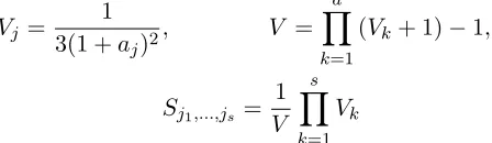
Sj1,...,js =
Vj1,...,js
V (27)
where 1 ≤ j1 < . . . < js ≤ d and s = 1, . . . , d. Thus, Sj = Vj/V is called the first order
sensitivity index (or the main effect) for factor X(j), which measures the main effect of X(j)
on the output Y, the second order index Sjl = Vjl/V, for j 6= l, is called the second order sensitivity index expresses the sensitivity of the model to the interaction between variables
X(i) and X(j) on Y and so on for higher orders effects. The decomposition in (25) has the useful property that all sensitivity indices sum up to one.
p
The total sensitivity index (or total effect) of a given factor is defined as the sum of all the sensitivity indices involving the factor in question.
STj = X
l#j
Sl (29)
where #j represents all the Sj1,...,js terms that include the index j. Total sensitivity indices measure the part of output variance explained by all the effects in which it plays a role. Note however that the sum of all STj is higher than one because interaction terms are counted several times. It is important to note that total sensitivity indices can be computed by a single multidimensional integration and do not require computing all high order indices (see Sobol (1993)). Then comparing the total effect indices provides information about influential parameters.
GSA enables to explain the variability of the output response as a function of the input param-eters through the definition of total and partial sensitivity indices. The computation of these indices involves the computation of several multidimensional integrals that are estimated by Monte Carlo method and thus requires huge random samples. For this reason GSA techniques are prohibitive if used directly using the computer code (fluid flow simulator for example).
3.2. Global sensitivity analysis using COSSO
It has been shown in the previous section that when the input vector components are inde-pendently distributed (andX∈[0,1]d), the component functions in the ANOVA decomposition
are orthogonal and contain relevant information on the input/output relationships. Moreover, the total variance V of the model can be decomposed into its input variable contributions. Using the variance decomposition (25) and the COSSO solution form (6) we have
V ≈
Let us consider aN i.i.d random sample from the distribution ofX, say{zi= (zi1, . . . , zid)
Hence the main effect indices (first order sensitivity indices) are estimated as
b
Sj = Vjb b
V (33)
where Vb is the total variance estimation. The estimation of Vjl are given by
b
Thus, the second order indices are estimated by
b
Since we assume that a truncated form of ANOVA decomposition provides a satisfactory approximation of the model, the total effect indices estimation is given by
b
Notice that to compute all the indices (main effect, interaction and total effect) we need only
N evaluations of the meta-model.
4. Simulations
The present section is focused on studying the empirical performance of the four different versions of COSSO estimate and compares it to the GP method. The four version of COSSO are COSSO-IPS, COSSO-AIPS, COSSO-NN-LARS and COSSO-solver which use a standard convex optimizer (Matlab code developed by the COSSO’s authors Lin and Zhang (2006)). The empirical performance of estimators will be measured in terms of prediction accuracy and global sensitivity analysis (GSA). The measure of accuracy is given byQ2 defined as
Q2= 1−
where yi denotes the ith test observation of the test set, ¯y is their empirical mean andfb(xi)
is the predicted value at the design point xi. We also compare the methods for different
ex-perimental design sizes, uniformly distributed on [0,1]d and built by Latin Hypercube Design procedure (McKay et al., 1979) with maximin criterion (Santner et al., 2003) (maximinLHD). For each setting of each test example, we run 50 times and average. Thus we define the quan-tity ¯Q2 = 1/50P50k=1Qk2.
Concerning the performance in terms of GSA, we will study the accuracy of the total effect indices estimation. Furthermore, we will study the size effect of the sample used to estimate the total effect indices by Monte-Carlo integration. We will compare the results to those ob-tained by Sobol’s method described in Sobol (1993) and Saltelli et al. (2000) and using GP meta-modeling procedure.
To fit COSSO models using a standard convex optimizer we have used the matlab code de-veloped by the COSSO’s authors Yi Lin and Hao Helen Zhang. COSSO-IPS, COSSO-AIPS and COSSO-NN-LARS are adapted versions of the original Matlab code. The GP code was implemented using R with a generalized power exponential Family (Busby, 2008).
4.1. Example 1
Consider the g-Sobol function, which is strongly nonlinear and is described by a non-monotonic relationship. Because of its complexity and the availability of analytical sensitivity indices, this function is a well-known test case in the studies of GSA. Figure 1 illustrates the g-Sobol function against the two most influential parameters X(1) and X(2). The g-Sobol function (Saltelli et al. (2000)) is defined for 8 inputs factors as
gSobol(X(1), . . . , X(8)) =
variability of the model output is represented by the weighting coefficient ak. The lower this
coefficient ak, the more significant the variableX(k). For example:
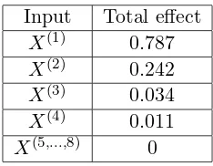
The analytical values of Sobol’s indices are given by (Sudret, 2008)
Vj =
are shown in table (1).
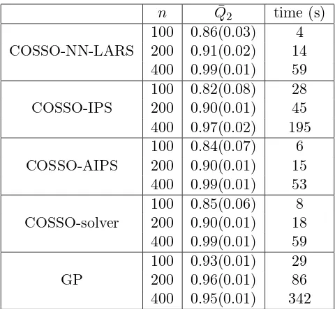
4.1.1. Assessment of the prediction accuracy
Table 2 summarizes the results for the 50 realizations of the g-Sobol model with three different experimental design sizes (n = 100, n = 200 and n = 400). It appears that for this example the GP outperforms all of the COSSO versions for n = 100 and n = 200. However, when the experimental design size increases, the performance of the GP does not get
X1
0.0
0.2
0.4
0.6
0.8
1.0
X2
0.0 0.2
0.4 0.6
0.8 1.0
f(X)
0.0 0.5 1.0 1.5 2.0
Figure 1: Plot of g-Sobol function versus inputsX(1) andX(2)with other inputs fixed at 0.5
Input Total effect
X(1) 0.787
X(2) 0.242
X(3) 0.034
X(4) 0.011
X(5,...,8) 0
Table 1: Analytical values of the total effect indices of the g-Sobol function
much better while all the COSSO methods increase their accuracy by increasing the sample size. Indeed, for n= 400 the COSSO methods outperforms GP especially COSSO-NN-LARS, COSSO-AIPS and COSSO-solver, which have ¯Q2 quantity equal to 0.99 that indicates that
those meta-models explain 99% of the model variance. All the COSSO versions provide quite similar result for this example. Moreover, as expected, the AIPS method is clearly faster than IPS. Notice that even if the NN-LARS provides the entire path of the solution, the COSSO-NN-LARS method has the same computational cost as COSSO-AIPS and COSSO-solver, the reason of that is the choice of the best model byv-fold-cross-validation which is computationally costly.
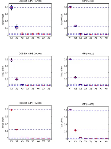
4.1.2. Global sensitivity analysis
In this subsection, we apply the COSSO-AIPS method in order to estimate the total ef-fect indices. The choice of COSSO-AIPS instead of other COSSO was motivated by the good performance of the method and it fast execution. We first focus on the robustness of the size effect of the sample used to estimate the indices. To this end, we repeated the experiment
n Q¯2 time (s)
COSSO-NN-LARS
100 0.86(0.03) 4 200 0.91(0.02) 14 400 0.99(0.01) 59
COSSO-IPS
100 0.82(0.08) 28 200 0.90(0.01) 45 400 0.97(0.02) 195
COSSO-AIPS
100 0.84(0.07) 6 200 0.90(0.01) 15 400 0.99(0.01) 53
COSSO-solver
100 0.85(0.06) 8 200 0.90(0.01) 18 400 0.99(0.01) 59
GP
100 0.93(0.01) 29 200 0.96(0.01) 86 400 0.95(0.01) 342
Table 2: Q2results from the g-Sobol function. The estimated standard deviation ofQ2 is given in parentheses.
100 times with two different sample size N = 500 and N = 5000 built using maximinLHD. We estimate the indices using a meta-model build by COSSO-AIPS of an experimental design of size n= 400 and having a Q2 equal to 0.99. We compare the results to those obtained by
Sobol’s method of indices estimation based on meta-model build by GP on an experimental design of sizen= 400 and having aQ2equal to 0.96. As introduced previously Sobol’s methods
to estimate the total effect needs 2 samples, thus we build, using a maximinLHD procedure, 200 samples of two sizes: N = 500 and N = 5000. Figure 2 summarizes the results for the 100 different samples and the two sizes (N = 500 and N = 5000). Each panel is a boxplot of the 100 estimations of the total effect index STb j, j = 1, . . . ,8. Dashed lines are drawn at the corresponding analytical values of the total effects indices. We see that our direct method of indices estimation based on COSSO procedure is more robust than Sobol’s one using the GP meta-model, especially when the sample size is small (N = 500). Moreover our method needs only N evaluation of the COSSO-AIPS meta-model while Sobol’s method needs 2N d
evaluations of GP meta-model (forN = 5000, 80000 evaluations are used).
To study the performance of the total effect indices estimations versus the sizes of the ex-perimental design we compute the indices, using sample of size N = 5000, for each of the 50’s realizations and for the three different experimental design sizes (n= 100, n= 200 and
n= 400). Figure 3 summarizes the results, each panel is a boxplot of the 50 estimations ofSbTj,
j= 1, . . . ,8. Dashed lines are drawn at the corresponding analytical values of the total effects indices. As expected the estimations based on GP meta-models outperforms those based on COSSO-AIPS for n= 100 and n = 200, which is due to the better performances in terms of
Q2 of the GP for these experimental design sizes. Nevertheless, for n= 400 the estimations
based on COSSO-AIPS are better than those based on GP.
0 0.2 0.4 0.6 0.8
X1 X2 X3 X4 X5 X6 X7 X8
Total effect
COSSO−AIPS (N=500)
0 0.2 0.4 0.6 0.8
X1 X2 X3 X4 X5 X6 X7 X8
Total effect
GP (N=500)
0 0.2 0.4 0.6 0.8
X1 X2 X3 X4 X5 X6 X7 X8
Total effect
COSSO−AIPS (N=5000)
0 0.2 0.4 0.6 0.8
X1 X2 X3 X4 X5 X6 X7 X8
Total effect
GP (N=5000)
Figure 2: Total effect indices vs. sample effect (example 1)
0 0.2 0.4 0.6 0.8
X1 X2 X3 X4 X5 X6 X7 X8
Total effect
COSSO−AIPS (n=100)
0 0.2 0.4 0.6 0.8
X1 X2 X3 X4 X5 X6 X7 X8
Total effect
GP (n=100)
0 0.2 0.4 0.6 0.8
X1 X2 X3 X4 X5 X6 X7 X8
Total effect
COSSO−AIPS (n=200)
0 0.2 0.4 0.6 0.8
X1 X2 X3 X4 X5 X6 X7 X8
Total effect
GP (n=200)
0 0.2 0.4 0.6 0.8
X1 X2 X3 X4 X5 X6 X7 X8
Total effect
COSSO−AIPS (n=400)
0 0.2 0.4 0.6 0.8
X1 X2 X3 X4 X5 X6 X7 X8
Total effect
GP (n=400)
Figure 3: Total effect indices vs. experimental design size effect (example 1)
4.2. Example 2
Let consider the same example that has been used in the COSSO paper (Example 3). This 10 dimensional regression problem is defined as
f(X) =g1(X(1))+g2(X(2))+g3(X(3))+g4(X(4))+g1(X(3)+X(4))+g2(
X(1)X(3)
2 )+g3(X
(1)X(2))
(38) where
g1(t) =t; g2(t) = (2t−1)2; g3(t) =
sin(2πt) 2−sin(2πt);
g4(t) = 0.1 sin(2πt) + 0.2 cos(2πt) + 0.3 sin2(2πt) + 0.4 cos3(2πt) + 0.5 sin3(2πt)
Therefore X(5), . . . , X(8) are uninformative. This analytical model is fast enough to evaluate
so we can calculate the total effect indices with great precision. Thus the reference values of the indices are computed by direct Monte-Carlo simulation using Sobol’s method (with
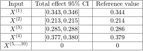
N = 250000, which correspond to 5.106 evaluations of the example 2). Table 3 shows 95% confidence intervals (95% CI) provided by 100 different samples and the chosen reference values
Input Total effect 95% CI Reference value
X(1) [0.343,0.346] 0.344
X(2) [0.213,0.215] 0.214
X(3) [0.285,0.288] 0.286
X(4) [0.377,0.380] 0.379
X(5,...,10) 0 0
Table 3: 95% CI and the reference values of the total effect indices for the example 2
4.2.1. Assessment of the prediction accuracy
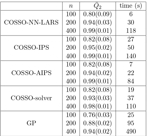
Table 4 summarizes the results for the 50 realizations of the example 2 model with three different experimental design sizes (n = 100, n = 200 and n = 400). Here we see that for all versions and for all sizes of experimental designs the COSSO method outperforms GP. The accuracy for all methods improves as the experimental design increases. Notice that the COSSO-AIPS method is the fastest one, especially with a large experimental design size as opposed to the GP, which is the slowest method.
4.2.2. Global sensitivity analysis
As in the previous subsection, we apply the COSSO-AIPS method in order to estimate the total effect indices. We first focus on the size effect of the sample used to estimate the indices. Thus we build, using a maximinLHD procedure, 100 samples of two sizes: N = 500 and N = 5000; then we estimate the indices using a meta-model built by COSSO-AIPS of an experimental design of size n= 400 and having a Q2 equal to 0.99. We compare the results
to those obtained by Sobol’s method of indices estimation based on meta-model built by GP on an experimental design of size n= 400 and having a Q2 equal to 0.95. We build, using a
maximinLHD procedure, 200 samples of two sizes: N = 500 andN = 5000.
n Q¯2 time (s)
COSSO-NN-LARS
100 0.80(0.09) 6 200 0.94(0.03) 30 400 0.99(0.01) 118
COSSO-IPS
100 0.82(0.08) 27 200 0.95(0.02) 50 400 0.99(0.01) 140
COSSO-AIPS
100 0.82(0.08) 7 200 0.94(0.02) 22 400 0.99(0.01) 84
COSSO-solver
100 0.82(0.08) 19 200 0.93(0.03) 37 400 0.98(0.01) 110
GP
100 0.76(0.03) 25 200 0.88(0.02) 95 400 0.94(0.02) 490
Table 4:Q2 results from example 2. The estimated standard deviation ofQ2 is given in parentheses.
Figure 6 shows the results obtained by the 100 different samples and for the two sizes (N = 500 and N = 5000). Each panel is a boxplot of the 100 estimations of the total effect indicesSbTj,
j= 1, . . . ,10. Dashed lines are drawn at the corresponding reference values of the total effects indices. We see that our direct method of indices estimation based on COSSO method is more robust than Sobol’s one using the GP meta-model especially when the sample size is small (N = 500).
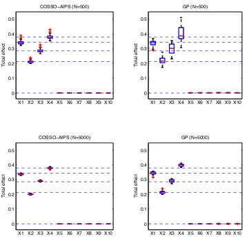
A summary of the indices estimation on 50 realizations and for the three different experimental design size (n = 100, n = 200 and n = 400) is shown in figure 5. Each panel is a boxplot of the 50 estimations of STb j, j = 1, . . . ,10. Dashed lines are drawn at the corresponding analytical values of the total effects indices. It appears that the indices estimation using COSSO-AIPS suffers more from the small experimental design sizes than GP, especially for those indices corresponding to the uninformative inputs. However, as the sample size increases, our COSSO-AIPS method have performs better than Sobol’s with GP.
4.3. Example 3
This third example is a high dimensional model withd= 20. This model is defined as
f(X) =g1(X(1)) +g2(X(2)) +g3(X(3)) +g4(X(4)) + 1.5g2(X(8)) + 1.5g3(X(9))
+ 1.5g4(X(10)) + 2g3(X(11)) + 1.5g4(X(12)) +g3(X(1)X(2)) +g2(X
(1)+X(3)
2 )
+g1(X(3)X(4)) + 2g3(X(5)X(6)) + 2g2(
X(5)+X(7)
2 )
where the functionsg1,g2,g3andg4are the same as for example 2. Notice thatX(13), . . . , X(20)
are uninformative. The reference values of the total effect indices are computed by direct Monte-Carlo simulation using Sobol’s method (with N = 250000, which corresponds to 5.106
0 0.1 0.2 0.3 0.4 0.5
X1 X2 X3 X4 X5 X6 X7 X8 X9 X10
Total effect
COSSO−AIPS (N=500)
0 0.1 0.2 0.3 0.4 0.5
X1 X2 X3 X4 X5 X6 X7 X8 X9 X10
Total effect
GP (N=500)
0 0.1 0.2 0.3 0.4 0.5
X1 X2 X3 X4 X5 X6 X7 X8 X9 X10
Total effect
COSSO−AIPS (N=5000)
0 0.1 0.2 0.3 0.4 0.5
X1 X2 X3 X4 X5 X6 X7 X8 X9 X10
Total effect
GP (N=5000)
Figure 4: Total effect indices vs. sample effect (example 2)
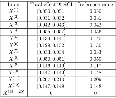
evaluations of the example 3 model). Table 7 shows 95% confidence intervals (95% CI) provided by 100 different samples and the chosen reference values.
4.3.1. Assessment of the prediction accuracy
Table 6 summarizes the results for the 50 realizations of the example 3 model with two different experimental design sizes (n= 200 andn= 400) build using maximinLHD procedure. For this example we choose to do not test COSSO-IPS since we shown with the previous tests that AIPS have better computational performance. It can be seen that for this model GP has a bad performance for the both sizes of the experimental design. Concerning the COSSO methods we can see that as the size of the experimental design increases, both COSSO-AIPS and COSSO-solver provide increasingly accurate estimates. However, we can note that COSSO-NN-LARS does not increase its performance as others and as one would expect. As for previous examples, notice that COSSO-AIPS is the fastest method especially comparing to
0
Figure 5: Total effect indices vs. experimental design size effect (example 2)
Input Total effect 95%CI Reference value
X(1) [0.050,0.051] 0.050
X(2) [0.031,0.032] 0.031
X(3) [0.042,0.043] 0.042
X(4) [0.055,0.057] 0.056
X(5) [0.139,0.141] 0.140
X(6) [0.129,0.132] 0.130
X(7) [0.033,0.034] 0.033
X(8) [0.050,0.051] 0.050
X(9) [0.116,0.119] 0.117
X(10) [0.147,0.149] 0.148
X(11) [0.207,0.210] 0.209
X(12) [0.147,0.149] 0.148
X(13,...,20) 0 0
Table 5: 95% CI and the reference values of the total effect indices for example 3.
COSSO-solver and GP.
n Q¯2 time (s)
COSSO-NN-LARS 200 0.73(0.10) 120 400 0.75(0.08) 281
COSSO-AIPS 200 0.78(0.08) 78 400 0.94(0.04) 274
COSSO-solver 200 0.78(0.09) 355 400 0.94(0.02) 720
GP 200 0.40(0.05) 240 400 0.56(0.03) 1105
Table 6:Q2 results from example 3. The estimated standard deviation ofQ2 is given in parentheses.
4.3.2. Global sensitivity analysis
In this section, total effect indices are computed using COSSO-AIPS. Here we do not compare the results to those using Sobol’s method with GP meta-model, because of its bad prediction performance (see Table 6 ). As previously, we first study the effect of the sample size N on indices estimations. Thus, we build using maximinLHD procedure, 100 samples of two sizes N = 500 and N = 5000 and we compute the indices using our direct method based on predictive COSSO-AIPS meta-model (Q2 = 0.98). We can see in the figure 6 that those
estimates are close to the reference values of the indices and that robustness of estimations increases by increasing N, nevertheless withN = 500 estimations are still quite good.
Table 7 summarize the results from using meta-models build with the two different sizes of experimental design (n= 200 and n= 400). As one would expect the accuracy of the indices estimations improves as the experimental design increases (in other words as the predictivity
improves). This study was done using the 50 meta-models used in the previous section using a N = 5000 sample to compute the total effect indices.
5. The petroleum reservoir test cases
5.1. PUNQS test case
5.1.1. Reservoir model description
The PUNQS case is a synthetic reservoir model taken from a real field located in the North Sea. The PUNQS test case, which is qualified as a small-size model, is frequently used as a benchmark reservoir engineering model for uncertainty analysis and for history-matching studies.
The geological model contains 19×28×5 grid blocks, 1761 of which are active. The reservoir is surrounded by a strong aquifer in the North and the West, and is bounded to the East and South by a fault. A small gas cap is located in the centre of the dome shaped structure. The geological model consists of five independent layers, where the porosity distribution in each layer was modelled by geostatistical simulation. The layers 1, 3, 4 and 5 are assumed to be of good quality, while the layer 2 is of poorer quality. The field contains six production wells located around the gas-oil contact. Due to the strong aquifer, no injection wells are required. For more detailed description on the model, see PUNQS (1996). Twenty uncertain parameters uniformly distributed and independent, are considered in this study:
• DensityGas U[0.8; 0.9] Kg/m3: gas density
• DensityOil U[900; 950]Kg/m3: oil density
• M P H U[0.5; 1.5]: horizontal transmissibility multipliers for each layers (from 1 to 5)
• M P V U[0.5; 5]: vertical transmissibility multipliers for each layers (from 1 to 5)
• P ermAqui1 U[100; 200] mD: analytical permeability of the aquifer 1
• P ermAqui2 U[100; 200] mD: analytical permeability of the aquifer 2
• P oroAqui1U[0.2; 0.3]: analytical porosity of the aquifer 1
• P oroAqui2U[0.2; 0.3]: analytical porosity of the aquifer 2
• SGCR U[0.02; 0.08]: critical gas saturation
• SOGCR U[0.2; 0.3]: critical oil gas saturation; largest oil saturation at which oil is immobile in gas
• SOW CR U[0.15; 0.2]: critical oil water saturation; largest oil saturation at which oil is immobile in water
• SW CR U[0.2; 0.3]: critical water saturation
For this study we focus on an objective function output, defined as:
OF(X) = (f(X)−d)
TC−1
D (f(X)−d)
2 (39)
0 0.05 0.1 0.15 0.2 0.25
X1 X2 X3 X4 X5 X6 X7 X8 X9 X10 X11 X12 X13 X14 X15 X16 X17 X18 X19 X20
Total effect
N=500
0 0.05 0.1 0.15 0.2 0.25
X1 X2 X3 X4 X5 X6 X7 X8 X9 X10 X11 X12 X13 X14 X15 X16 X17 X18 X19 X20
Total effect
N=5000
Figure 6: Total effect indices vs. sample effect (example 3)
Input Reference value n= 200 n= 400
X(1) 0.050 0.035(0.017) 0.047(0.008)
X(2) 0.031 0.022(0.019) 0.023(0.012)
X(3) 0.042 0.021(0.019) 0.040(0.015)
X(4) 0.056 0.029(0.022) 0.052(0.008)
X(5) 0.140 0.127(0.033) 0.124(0.009)
X(6) 0.130 0.107(0.051) 0.120(0.011)
X(7) 0.033 0.034(0.028) 0.034(0.006)
X(8) 0.050 0.041(0.034) 0.054(0.006)
X(9) 0.117 0.146(0.018) 0.118(0.011)
X(10) 0.148 0.172(0.025) 0.145(0.008)
X(11) 0.209 0.248(0.05) 0.210(0.011)
X(12) 0.148 0.158(0.026) 0.144(0.009)
X(13) 0 0.003(0.004) 0.001(0.001)
X(14) 0 0.002(0.004) 0.001(0.001)
X(15) 0 0.004(0.006) 0.001(0.002)
X(16) 0 0.001(0.003) 0.002(0.001)
X(17) 0 0.003(0.003) 0.001(0.001)
X(18) 0 0.001(0.002) 0.001(0.002)
X(19) 0 0.003(0.004) 0.001(0.002)
X(20) 0 0.004(0.009) 0.001(0.002)
Table 7: Total effect indices vs. experimental design size effect (example 3). The estimated standard deviation of the total effect index are given in parentheses.
Figure 7: Top structure map of the reservoir field (PUNQS test case).
where CD is the covariance matrix of the observed data and dthe observed data. This OF is
given by equation (39) and represents the mismatch between observed and simulated data. The observed data is synthetically generated using a random value for the uncertain parameters in the simulator and adding noise (10% of the average value of each time series) to the results. This data consists in time series given with two months frequency during the first 6 years for the following simulator outputs: Gas Oil Ratio, Bottom Hole Pressure, Oil Production Rate, and Water Cut. To define the weights in the objective function definition, we consider independent measurement errors for each time dependent output. This error was taken to be equal to 10% of the average value of each time series.
5.1.2. Assessment of the prediction accuracy
Each of the input range has been rescaled to the interval [0,1] and the reservoir simulator is run on two experimental designs of size n = 200 and n = 400, which were built using maximinLHD. Then we construct meta-models using AIPS, C0SSO-solver, COSSO-NN-LARS and GP. In order to estimateQ2 the simulator was run at an additional sample set
of size ntest = 500. Table 8 shows the results of this study. We see that for this test case GP
outperforms COSSO’s methods, but differences between Q2 given by the used methods are
small when the design size is n= 400. In addition, as previously shown COSSO-AIPS is less time consuming than others especially if we compare it with GP. Consequently COSSO and particularly COSSO-AIPS is well adapted to perform GSA.
n Q2 time (s)
COSSO-NN-LARS 200 0.67 200 400 0.81 450
COSSO-AIPS 200 0.69 70 400 0.82 300
COSSO-solver 200 0.67 280 400 0.81 700
GP 200 0.75 402
400 0.84 794
Table 8: PUNQS modelQ2 results
5.1.3. Global sensitivity analysis
Here we use COSSO-AIPS and GP to produce meta-models which are built using the experimental design of size n = 400. To compute the total effect and main effect indices via COSSO-AIPS we use a sample of sizeN = 5000 and two samples of the same size for the case using GP. We provided here the main effect indices to show the reader the importance of the interaction effects in this model. Tables 9 shows the computed indices, thus we can see that the main effect and the interactions ofM P H5 explain more than 65% of the model variance, then we have a group of five inputs (SW CR, M P H1, SOGCR, SGCR and P ermAqui1 ) with relatively important effects and a group of five or six (depending on the method used) inputs with poor importance (0.05 > SbTj > 0.01). While the remaining are considered as uninformative. The GSA results using COSSO-AIPS and GP are almost equivalent, which was expected knowing that their Q2 are close.
5.2. IC Fault Model
5.2.1. Reservoir model description
The geological model consists of six layers of alternating good and poor quality sands (see Figure 8 ). The three good quality layers have identical properties, and three poor quality layers have different set of identical properties. The thickness of the layers has arithmetic progression, with the top layer having a thickness of 12.5 feet, the bottom layer a thickness of 7.5 feet, and a total thickness of 60 feet. The width of the model is 1000 feet, with a simple fault at the mid-point, which off-sets the layers. There is a water injector well at the left-hand edge, and a producer well on the right-hand edge. Both wells are completed on all layers, and operated at a fixed bottom hole pressures.
The simulation model is 100×12 grid blocks, with each geological layer divided into two simu-lation layers with equal thicknesses, each grid block is 10 feet wide. The model is constructed such that the vertical positions of the wells are kept constant and equal, even when different fault throws are considered. The well depth is 8325 feet to 8385.
The porosity and permeabilities in each grid block were randomly drawn from uniform distri-butions with no correlations. The range for the porosities was ±10 of the mean value, while range for the permeabilities was±1 of the mean value. The means for the porosities were 0.30 for the good quality sand and 0.15 for the bad quality sand. The means of the permeabilities were 158.6 mD for the good quality sand and 2.0 mD for the poor quality sand.
This simplified reservoir model has three uncertain input parameters, corresponding to the
GP
Input Total effect Main effect
M P H5 0.656 0.396
Input Total effect Main effect
M P H5 0.664 0.402
DensityGas 0.001 0
M P H2 0 0
M P H4 0 0
Table 9: GSA from PUNQS model
fault throw h, the good and the poor sand permeability multipliers kg and kp. The three parameters are selected independently from uniform distributions with ranges: h ∈ [0,60]
kg∈[100,200] andkp ∈[0,50]. The analysed output is in this test case the oil production rate
Qop at 10 years. Figure 9 illustrates this output against kg and kp at a fixed high value ofh. For more detailed description on the IC Fault model, see Tavassoli et al. (2004).
5.2.2. Assessment of the prediction accuracy
The simulator is run on four experimental designs of size n = 100, n = 200, n = 400 and n = 1600 generated by maximinLHD procedure. Then we construct meta-models using COSSO-AIPS and GP. In order to estimateQ2, the simulator was run at an additional sample
set of size ntest = 25000. Table 10 shows the results of this study. Clearly, COSSO-AIPS
outperforms GP in this test case, however an experimental design of size n= 400 is necessary to provide a reasonably accurate estimate. Moreover, we can note that as the experimental design increases the accuracy of COSSO-AIPS estimate increases, this is not the case for GP as remarked in Example 1. Indeed, by increasing the design from 200 to 400 instead of improving, the estimate becomes worse in terms of predictivity. Even if there are only three uncertain inputs in this test case, the approximation of the input/output relation is a complicated problem, this is due to the presence of the fault that provide discontinuities in the model.
Figure 8: IC Fault Model
Figure 9: Oil production rate after 10 years vs. kg and kp at a fixed high value of h (obtained with 1000 simulations)
5.2.3. Global sensitivity analysis
As for PUNQS test case we use COSSO-AIPS and GP to produce meta-models which are built using the experimental design of size n = 1600. To compute the total effect and main effect indices via COSSO-AIPS we use a sample of size N = 5000 and two samples of the same size for the case using GP. Tables 11 shows the computed indices. Following the GSA
n Q2 time (s)
COSSO-AIPS
100 0.34 1 200 0.63 4 400 0.72 15 1600 0.81 280
GP
100 0.33 8 200 0.57 25 400 0.52 63 1600 0.66 1128
Table 10: IC fault modelQ2 results
results produced via COSSO-AIPS, we can see that the variance of the oil production rate mainly depend on the fault throwhand the poor sand permeabilitykp. With respect to GSA,
results produced via GP gives more interaction effect to the good sand permeability kg than COSSO-AIPS. The betterQ2 of COSSO-AIPS suggests that its GSA results are more robust.
GP
Input Total effect Main effect
h 0.381 0.100
kg 0.173 0.021
kp 0.809 0.596
COSSO-AIPS
Input Total effect Main effect
h 0.375 0.225
kg 0.030 0.011
kp 0.733 0.586
Table 11: GSA from IC fault model
6. Conclusion
In this work, we presented the COSSO regularized nonparametric regression method, which is a model fitting and variable selection procedure. One of the COSSO’s algorithm steps is the NNG optimization problem. The original COSSO algorithm uses classical constrained optimization techniques to solve the NNG problem, these techniques are efficient but time consuming, especially with high dimensional problems (as empirically shown) and with big size of experimental design (high number of observations). A new iterative algorithm was de-veloped, so-called IPS with its accelerated version (AIPS). Based on the Landweber iterations these procedures are conceptually simple and easy to implement.
We also applied the NN-LARS algorithm to COSSO that, as expected, has competitive com-putation time performance comparing to the original COSSO (COSSO-solver). We empirically show that COSSO based on the AIPS algorithm is the fastest COSSO version.
Moreover, we used the ANOVA decomposition basis of the COSSO to introduce a direct method to compute the Sobol’ indices. We applied COSSO to the problem of GSA for several analytical models and reservoir synthetic test cases, and we compared its performance to GP method combined with Sobol’ Monte-Carlo method. For all the test cases COSSO shows very competitive performances, especially the COSSO-AIPS version, for which the computational
gain was significant compared to COSSO-solver and GP. Consequently, COSSO-AIPS consti-tutes an efficient and practical approach to GSA.
Acknowledgements
The authors are grateful to Professor Anestis Antoniadis for many useful suggestions and helpful discussions.
Berlinet, A., Thomas-Agnan, C., 2003. Reproducing Kernel Hilbert Spaces in Probability and Statistics. Kluwer Academic Publishers.
Bioucas-Dias, J. M., Figueiredo, M. A. T., 2007. A new twist: two-step iterative shrink-age/thresholding algorithms for image restoration. IEEE Transactions on Image Processing 16, 2992 – 3004.
Blatman, G., Sudret, B., 2010. Efficient computation of global sensitivity indices using sparse polynomial chaos expansions. Reliability Engineering and System Safety 95, 1216–1229.
Breiman, L., 1995. Better subst regression using the nonnegative garrote. Technometrics 37, 373–384.
Busby, D., 2008. Hierarchical adaptive experimental design for gaussian process emulators. Reliability Engineering and System Safety 94, 1183–1193.
Busby, D., Farmer, C. L., Iske, A., 2007. Hierarchical nonlinear approximation for experimental design and statistical data fitting. SIAM J. Sci. Comput 29 (1), 49–69.
Daubechies, I., Fornasier, M., Loris, I., 2008. Accelerated projected gradient method for linear inverse problems with sparsity constraints. Journal of Fourier Analysis and Applications 14 (5-6), 764–792.
Efron, B., Hastie, T., Johnstone, I., Tibshirani, R. J., 2004. Least angle regression. The annals of statistics 32, 407–499.
Landweber, L., 1951. An iterative formula for fredholm integral equations of the first kind. American journal of mathematics 73, 615–624.
Lin, Y., Zhang, H., 2006. Component selection and smoothing in smoothing spline analysis of variance models. Annals of Statistics 34(5), 2272–2297.
Marrel, A., Ioss, B., Dorpe, F. V., Volkova, E., 2008. An efficient methodology for model-ing complex computer codes with gaussian processes. Computational Statistics and Data Analysis 52, 4731–4744.
McKay, M. D., Beckman, R. J., Conover, W. J., 1979. A comparison of three methods for selecting values of input variables in the analysis of output from a computer code. Techno-metrics 21, 239–245.
Piana, M., Bertero, M., 1997. Projected landweber method and preconditioning. Inverse Prob-lems 13, 441–463.
PUNQS, 1996. Production forecasting with uncertainty quantification. website.
URLhttp://www.fault-analysis-group.ucd.ie/Projects/PUNQ.html
Sacks, J., Welch, W. J., Mitchell, T. J., Wynn, H. P., 1989. Design and analysis of computer experiments. Statistical science 4, 409–435.
Saltelli, A., Chan, K., Scott, M., 2000. Sensitivity analysis. Wiley.
Santner, T. J., Williams, B. J., Notz, W. I., 2003. The design and analysis of computer experiments. Springer.
Sobol, I., 1993. Sensitivity estimates for nonlinear mathematical models. Mathematical Mod-elling and Computational Experiments 1, 407–414.
Storlie, C. B., Bondell, H. D., Reich, B. J., Zhang, H., 2008. Surface estimation, variable selection, and the nonparametric oracle property. Journal of the Royal Statistical Society : Serie B.
Storlie, C. B., Helton, J. C., 2008a. Multiple predictor smoothing methods for sensitivity analysis: Description of techniques. Reliability engineering and system safety 93, 28–54.
Storlie, C. B., Helton, J. C., 2008b. Multiple predictor smoothing methods for sensitivity analysis: examples results. Reliability Engineering and System Safety 93, 57–77.
Storlie, C. B., Swiler, L. P., Helton, J. C., Sallaberry, C. J., 2009. Implementation and eval-uation of nonparametric regression procedures for sensitivity analysis of computationally demanding models. Reliability engineering and systems safety 94, n 11, 1735–1763.
Sudret, B., 2008. Global sensitivity analysis using polynomial chaos expansions. Reliability Engineering and System Safety 93, 964–979.
Tavassoli, Z., Carter, J. N., King, P. R., 2004. Errors in history matching. SPE Journal, 352– 361.
Tibshirani, R. J., 1996. Regression shrinkage and selection via the lasso. Journal of Royal Statistical Society Series B 58, 267–288.
Touzani, S., Busby, D., 2011. Multivariate wavelet kernel regression method.
URLhttp://hal.archives-ouvertes.fr/hal-00616280/fr/
Wahba, G., 1990. Spline models for observational data. SIAM.
Yuan, M., Lin, Y., 2007. On the nonnegative garrote estimator. Journal of Royal Statistical Society Series B 69, 143–161.