DOI: 10.12928/telkomnika.v14.i3.3281 1024
Musical Genre Classification Using Support Vector
Machines and Audio Features
A.B. Mutiara*, R. Refianti , and N.R.A. Mukarromah
Faculty of Computer Science and Information Technology, Gunadarma University, Depok 16424, Indonesia Jl. Margonda Raya No.100, Depok 16424, Indonesia, fax +62-21-78
*corresponding author, e-mail: [email protected]
Abstract
The need of advance Music Information Retrieval increases as well as a huge amount of digital music files distribution on the internet. Musical genres are the main top-level descriptors used to organize digital music files. Most of work in labeling genre done manually. Thus, an automatic way for labeling a genre to digital music files is needed. The most standard approach to do automatic musical genre classi-fication is feature extraction followed by supervised machine-learning. This research aims to find the best combination of audio features using several kernels of non-linear Support Vector Machines (SVM). The 31 different combinations of proposed audio features are dissimilar compared in any other related research. Furthermore, among the proposed audio features, Linear Predictive Coefficients (LPC) has not been used in another works related to musical genre classification. LPC was originally used for speech coding. An experimentation in classifying digital music file into a genre is carried out. The experiments are done by extracting feature sets related to timbre, rhythm, tonality and LPC from music files. All possible combination of the extracted features are classified using three different kernel of SVM classifier that are Radial Basis Function (RBF), polynomial and sigmoid. The result shows that the most appropriate kernel for automatic musical genre classification is polynomial kernel and the best combination of audio features is the combina-tion of musical surface, Mel-Frequency Cepstrum Coefficients (MFCC), tonality and LPC. It achieves 76.6 % in classification accuracy.
Keyword: Support Vector Machine, Audio Features, Mel-Frequency Cepstrum Coefficients, Linear Predic-tive Coefficients
Copyrightc 2016 Universitas Ahmad Dahlan. All rights reserved.
1. Introduction
A standard approach for automatic musical genre classification is a feature extraction followed by supervised machine-learning. Feature extraction transforms the input data into a reduced representation set of features instead of the full size input. There are a lot of features that can be extracted from audio signals that may be related to main dimension of music including timbre, rhythm, pitch, tonality etc. In the case of genre classification, a rigorous selection of feature that can be used to distinguish one genre to another is a key factor in order to achieve great accuracy in classification result.
Several feature sets have been proposed to be used in representing genres. Those pro-posed feature sets are related to timbre, rhythm, pitch and tonality. Musical surface (spectral flux, spectral centroid, spectral rolloff, zero-crossings and low-energy) [1][2] and Mel-Frequency Cepstrum Coefficients (MFCC) [1][3] are used as features related to timbre. For rhythmic feature, strongest beat, strength of strongest beat and beat sum are used [4]. The features are obtained using the calculation of a Beat Histogram. Feature related to pitch uses accumulation of multiple pitch detection results in a Pitch Histogram. Based on research by [5], the use of this feature contributed a poor performance in classification accuracy. Features related to tonality are chro-magram, key strength and the peak of key strength [6]. There is another cepstral-based feature similar to MFCC called linear predictive coefficients (LPC). So far, LPC has not been used in works related to musical genre classification.
In order to do genre classification task, various supervised machine-learning classifier al-gorithm are used toward the extracted feature sets, such as, Linear Discriminant Analysis (LDA), k-Nearest Neighbor (kNN), Gaussian Mixture Model (GMM), and Support Vector Machines (SVM). The comparison among those algorithm has done by [7] resulting that SVM has the highest accu-racy level.
The need of advance Music Information Retrieval increases as well as a huge amount of digital music files distribution on internet. There are a lot of research and experiments of musical genre classification and the most standard approach is feature extraction followed by supervised machine-learning. Several feature sets and various supervised machine-learning algorithms have been proposed to do automatic musical genre classification. The problems of this research are: i) How to find the best combination of feature sets that are extracted from music file for automatic musical genre classification task?; ii) How to find the most appropriate kernel of non-linear SVM kernel method for automatic musical genre classification task?
The scopes of the research are : i) Genres that are used to classify music file are limited to ten genres that are blues, classical, country, disco, hiphop, jazz, metal, pop, reggae, and rock.; ii) Although there are many data set of music available online, at this research we use data set of music files from GTZAN [8], an online available data set that contains 1000 music files with duration of 30 seconds. Every 100 music file represents one genre.; iii) The music files are using 22050 Hz sample rate, mono channel, 16-bit and .wav format. iv) The following are software used in the research: Windows 7 Operating System, MATLAB R2009a, MIRtoolbox 1.5, jAudio 1.0.4, Weka 3.7.10
This research aims to find the best combination of feature sets and SVM kernel for auto-matic musical genre classification. To do this, an experimentation in classifying digital music file into a genre will be carried out. In the experiments, all possible combination of feature sets related to timbre, rhythm, tonality and LPC that are extracted from music files are used and classified us-ing three different kernel of SVM classifier. The classification accuracy of each experiment are then compared to determine the best among these trials.
2. Literature Review 2.1. Music Genre
Musical genres are categories that have arisen through a complex interplay of cultures, artists and market forces to characterize similarities between musicians or compositions and or-ganize music collections [9]. Nowadays, music genres are often used to categorize music on radio, television and especially internet.
There is not any agreement on musical genre taxonomy. Therefore, most of music indus-tries and internet music stores use different genre taxonomies when categorizing music pieces into logical groups within a hierarchical structure. For example, allmusic.com uses 531 genres, mp3.com uses 430 genres, and amazon.com uses 719 genres in their database. Pachet and Cazaly [10] tried to define a general taxonomy of musical genres but they eventually gave up and used self-defined two-level genre taxonomy of 20 genres and 250 subgenres in their Cuidado music browser [11].
There are studies to identify human ability to classify music into a genre. One of them is a study conducted by R.O. Gjerdigen and D. Perrot [12] that uses ten different genres, namely Blues, Classical, Country, Dance, Jazz, Latin, Pop, R&B, Rap, and Rock. The subjects of the study were 52 college students enrolled in their first year of psychology. The accuracy of the genre prediction for the 3 s samples was around 70%. The accuracy for the 2.5 s samples was around 40%, and the average between the 2.5 s classification and the 3 s classification was around 44%.
2.2. Automatic Music Genre Classification
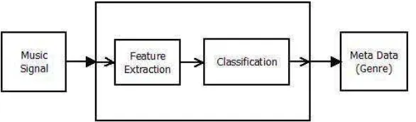
clas-sification part. The two steps can be clearly separated: the output of the feature extraction step is the input for the classification step [13]. The standard approach of music genre classification task can be seen in Figure 1.
Figure 1. Music genre classification standard approach.
2.3. Feature Extraction
Feature extraction is transforming the input data into a reduced representation set of fea-tures (also named as feafea-tures vector). If the feafea-tures extracted are carefully chosen it is expected that the features set will extract the relevant information from the input data in order to perform the desired task using this reduced representation instead of the full size input. In the case of audio signal, feature extraction is the process of computing a compact numerical representation that can be used to characterize a segment of audio [1].
To represent musical genre, some features extracted from audio signal that are related to timbre, rhythm and tonality are used. Those features can be divided as time-domain features and frequency-domain features. The calculation of time-domain features can be implemented directly to audio waveform (amplitude versus time). While for frequency-domain features, Fourier Trans-form is needed as the tools to obtain spectrum of audio (energy or magnitude versus frequency) that will be used to calculate the features. Fourier Transform is a mathematical transformation employed to transform signals from time domain into frequency domain. To compute the Fourier Transform digitally, the Discrete Fourier Transformation (DFT) algorithm is used, especially Fast Fourier Transform (FFT) and a Short Time Fourier Transformation (STFT). FFT is a faster version of DFT. The FFT utilizes some clever algorithms to do the same thing as the DFT, but in much less time. Evaluating DFT definition directly requiresO(N2)operations: there areN outputsX
k, and
each output requires a sum ofN terms. An FFT is any method to compute the same results in
O(N logN)operations. However, FFT have some drawbacks. FFT contains only frequency
infor-mation and no time inforinfor-mation is retained. Thus, it only works fine for stationary signal. It is not useful for analyzing time-variant, non-stationary signals since it only shows frequencies occurring at all times instead of specific times. To handle non-stationary signal, STFT is needed. The idea of STFT is framing or windowing the signal into narrow time intervals (possibly overlapping) and taking the FFT of each segment.
2.3.1. Features: Timbre, Rhythm and Tonality
The features used to represent timbre are based on standard features proposed for music-speech discrimination and music-speech recognition [5]. The features are spectral flux, spectral centroid, spectral rolloff, zero-crossings and low-energy that are grouped as musical surface features in [2], and also the mel-frequency cepstrum coefficients (MFCC). The timbre features are calculated based on the short-time Fourier transform which is performed frame by frame along the time axis. The detail of each feature will be elaborated in [15] about spectral centroid, [4] about spectral rolloff, [16] about spectral flux, [2] about zero crossing, [17] about MFCC.
calculated by taking the RMS of 256 windows and then taking the FFT of the result [4]. RMS is used to calculate the amplitude of a window. RMS can be calculated using the following equations:
RM S=
s PN
n=1x2n
N (1)
where N is the total number of samples (frames) provided in the time domain and x2
n is the
amplitude of the signal atnth sample.
Features related to tonality are proposed by [6]. Tonality used to denote a system of relationships between a series of pitches (forming melodies and harmonies) having a tonic, or central pitch class, as its most important (or stable) element. The features of tonality include, chromagram, key strength and peak of key strength.
2.3.2. Linear Predictive Coefficients (LPC)
The basic idea behind linear prediction is that a signal carries relative information. There-fore, the value of consecutive samples of a signal is approximately the same and the difference between them is small. It becomes easy to predict the output based on a linear combination of previous samples. For example, continuous time varying signal isxand its value at timetis the function ofx(t). When this signal is converted into discrete time domain samples, then the value of thenth sample is determined byx(n). To determine the value ofx(n)using linear prediction techniques, values of past samples such asx(n−1),x(n−2),x(n−3)..x(n−p)are used wherep
is the predictor order of the filter. This coding based on the values of previous samples is known as linear predictive coding [18].
2.4. Classification
In the terminology of machine learning, classification is considered an instance of super-vised learning, a learning where a training set of correctly identified observations is available. An algorithm that implements classification, especially in a concrete implementation, is known as a classifier.
2.4.1. Support Vector Machine
Support Vector Machine (SVM) is a technique for prediction task, either for classification or for regression. It was first introduced in 1992. SVM is member of supervised learning where categories are given to map instances into it by SVM algorithm.
Support Vector Machines are based on the concept of decision planes that define deci-sion boundaries. A decideci-sion plane is one that separates between a set of objects having different class memberships [19]. The basic idea of SVM is finding the best separator function (classi-fier/hyperplane) to separate the two kinds of objects. The best hyperplane is the hyperplane which is located in the middle of two object. Finding the best hyperplane is equivalent to maxi-mize margin between two different sets of object [20].
In real world, most classification tasks are not that simple to solve linearly. More complex structures are needed in order to make an optimal separation, that is, correctly classify new ob-jects (test cases) on the basis of the examples that are available (train cases). Kernel method is one of method to solve this problem. Kernels are rearranging the original objects using a set of mathematical functions. The process of rearranging the objects is known as mapping (transfor-mation). The kernel function, represents a dot product of input data points mapped into the higher dimensional feature space by transformationφ[19].
Linear operation in the feature space is equivalent to nonlinear operation in input space. Classification can become easier with a proper transformation [21]. There are number of kernels that can be used in SVM models. These include Polynomial, Radial Basis Function (RBF) and Sigmoid:
2. RBF:K(Xi,Xj) = exp(−γ|Xi−Xj|2)
3. Sigmoid:K(Xi,Xj) = tanh(γXi·Xj+C)
whereK(Xi,Xj) =φ(Xi)·φ(Xj), kernel function that should be used to substitute the dot product
in the feature space is highly dependent on the data.
2.4.2. K-Fold Cross Validation
For classification problems, the performance is measured of a model in terms of its error rate (percentage of incorrectly classified instances in the data set). In classification, two data sets are used: the training set (seen data) to build the model (determine its parameters) and the test set (unseen data) to measure its performance (holding the parameters constant). To split data into training and test set, a k-Fold Cross Validation is used.
K-Fold Cross Validation divides data randomly into k folds (subsets) of equal size. The k-1 folds are used for training the model, and one fold is used for testing. This process will be repeated k times so that all folds are used for testing. The overall performance is obtained by computing the average performance on the k test sets. This method effectively uses all the data for both training and testing. Typically k=5 or k = 10 are used for effective fold sizes [22].
2.4.3. Confusion Matrix
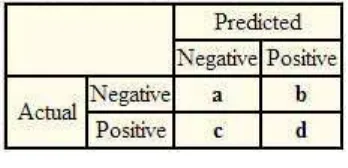
In the field of machine learning, a confusion matrix, is a specific table layout that allows visualization of the performance of an algorithm, typically a supervised learning one [23]. Each column of the matrix represents the instances in a predicted class, while each row represents the instances in an actual class.As seen on Figure 2, the entries in the confusion matrix have the following meaning:
Figure 2. Confusion matrix.
– a is the number of correct predictions that an instance is negative,
– b is the number of incorrect predictions that an instance is positive,
– c is the number of incorrect of predictions that an instance negative, and
– d is the number of correct predictions that an instance is positive.
3. Methodology
In this research, there are several steps to be done. These steps include data collection, feature extraction, data preprocessing, classification, and performance evaluation.
3.1. Data Collection, Feature Extraction, Data Preprocessing
data set consists of ten genres that are blues, classical, country, disco, hiphop, jazz, metal, pop, reggae, and rock where each genre is represented by 100 music files.
Feature extraction process is done toward music files in the data set. The features are calculated for every short-time frame of audio signal for time-domain features and are calculated based on short time fourier transform (STFT) for frequency-domain features. The features ex-tracted from the files. The process of feature extraction is done by utilizing MIRtoolbox [24], a MATLAB toolbox for musical feature extraction from audio and jAudio, a java feature extraction library [4][25].
The features data that are obtained from feature extraction phase are stored in two ARRF (Attribute-Relation File Format) file that are features.arff and features2 .arff. Before entering the classification stage, the data will be preprocessed so that the data are not separated in the differ-ent files.
3.2. Classification
In general, the process of classification in the experiments will use SVM classifier algo-rithm with kernel method and 10-fold cross validation strategy. The process is done by at first distributing the data set into 10 equal sized sets. 9 sets (set 2 to 10) are used as training set to generate classifier model with SVM classifier. The model is tested to the set 1 to measure its accuracy. In second iteration, set 2 will be used as testing set and set 1, 3 to 10 will be used as training set. This process is iterated until 10 classifier models are produced and all set are used as testing set. The accuracy of the 10 classifier models are averaged to obtain overall accuracy. The process of classification will be undertaken by utilizing Weka [26] data mining software.
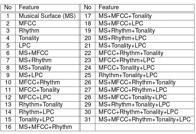
In the experiments, several classification processes will be done. Each classification pro-cess will use different combination of audio features as well as three different SVM kernel. Feature sets that will be experimented are grouped as Musical Surface (spectral flux, spectral centroid, spectral rolloff, zero-crossings, RMS energy and low-energy), MFCC, rhythm (strongest beat, beat sum and strength of strongest beat), tonality (chromagram, key strength and peak of key strength) and LPC. All possible combinations of these features can be seen at Table 1. SVM kernels used in the experiments are RBF, polynomial and sigmoid kernel. In the end, with multiplication of possible feature combinations and kernels used, there are 93 classification processes that will be tried out in the experiments.
Table 1. Possible Combination of the Feature Sets.
No Feature No Feature
1 Musical Surface (MS) 17 MS+MFCC+Tonality
2 MFCC 18 MS+MFCC+LPC
3 Rhythm 19 MS+Rhythm+Tonality
4 Tonality 20 MS+Rhythm+LPC
5 LPC 21 MS+Tonality+LPC
6 MS+MFCC 22 MFCC+Rhythm+Tonality
7 MS+Rhythm 23 MFCC+Rhythm+LPC
8 MS+Tonality 24 MFCC+Tonality+LPC
9 MS+LPC 25 Rhythm+Tonality+LPC
10 MFCC+Rhythm 26 MS+MFCC+Rhythm+Tonality
11 MFCC+Tonality 27 MS+MFCC+Rhythm+LPC
12 MFCC+LPC 28 MS+MFCC+Tonality+LPC
13 Rhythm+Tonality 29 MS+Rhythm+Tonality+LPC
14 Rhythm+LPC 30 MFCC+Rhythm+Tonality+LPC
15 Tonality+LPC 31 MS+MFCC+Rhythm+Tonality+LPC
3.3. Performance Evaluation
The performance of automatic musical genre classification in the experiments are eval-uated by classification accuracy that is obtained from each trial. A comparative analysis toward accuracy of 93 classification processes will be carried out in order to determine the best combina-tion of audio feature and the most appropriate kernel for automatic musical genre classificacombina-tion. The detail information of classification results will also be provided in the form of confusion ma-trix. It will show whether the music files are correctly classified into their genre or not. The rows represent the actual genre and the columns represent the predicted genre.
4. Results and Discussions 4.1. Feature Extraction Results
Feature extraction process is done toward 1000 music files in the data set which each 100 files represent one genre. The process is carried out in two step: fist step is utilizing MIRtoolbox as feature extraction tool and the second step is utilizing jAudio. In the first step, the code written in a MATLAB’s file called feature extraction.m is executed. In running this file, 21,874.955 seconds are elapsed. The statistical data of features related to timbre and tonality as well as the label of each file are obtained. In the end, the program generates features.arff file that contains the statistical information of features and file labels. In the second step, jAudio is used as feature extraction tool. Features extracted in this step are features related to timbre and tonality. The process takes 2.127 seconds to be accomplished. The output of this process are statistical information of features that is stored in features2.arff file.
4.2. Classification Results
The classification processes are done using Weka data mining software. The input is features final.arff file, a merger between features.arff and features2.arff file that are obtained from feature extraction stage. In this research, the experiments are carried out by classifying 31 differ-ent combination of feature sets using three differdiffer-ent kernels in SVM classifier for non linear data. The accuracy and detail information of classification results of the experiments will be provided in the following section.
4.2.1. Classification Accuracy of Experiments
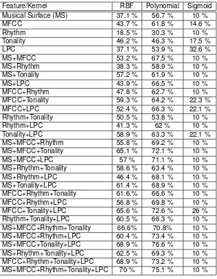
From the experiments conducted, overall performance results of 93 classification pro-cesses are obtained. The feature set of Musical Surface, MFCC, Rhythm, tonality and LPC and their combination are used. Table 2 compares the classification accuracy of various feature sets and their combinations using three kernels in SVM classifier: RBF, polynomial and sigmoid.
According to Table 2, it can be deduced that polynomial kernel is the most appropriate kernel for automatic musical genre classification since it always yields the best accuracy among all kernels for the same combination of features. The other two kernels are not suitable for this task. It is because RBF kernel does not give optimum result and sigmoid kernel does not completely suit with the data distribution of audio features.
The best accuracy is gained by the combination of MS+MFCC+Tonality+LPC features and the implementation of polynomial kernel with 76.6 % of correctly classified instances. The best accuracy is achieved by the combination of all feature sets excluding Rhythm feature. It is reasonable since in the experiment classification of individual feature set, Rhythm feature has the worst performance of all (30.3 %).
4.2.2. Classification Results in Confusion Matrix
Table 2. Accuracy of Classification Processes in the Experiments.
Feature/Kernel RBF Polynomial Sigmoid
Musical Surface (MS) 37.1 % 56.7 % 10 %
MFCC 43.7 % 61.8 % 14.6 %
Rhythm 18.5 % 30.3 % 10 %
Tonality 46.2 % 46.3 % 17.5 %
LPC 37.1 % 53.9 % 32.6 %
MS+MFCC 53.2 % 67.5 % 10 %
MS+Rhythm 38.3 % 58.9 % 10 %
MS+Tonality 57.2 % 61.9 % 10 %
MS+LPC 43.9 % 66.5 % 10 %
MFCC+Rhythm 47.8 % 62.7 % 10 %
MFCC+Tonality 59.3 % 64.2 % 22.3 %
MFCC+LPC 52.4 % 66.3 % 22.1 %
Rhythm+Tonality 50.5 % 53.8 % 10 %
Rhythm+LPC 41.3 % 62 % 10 %
Tonality+LPC 58.9 % 63.3 % 22.1 %
MS+MFCC+Rhythm 55.8 % 69.2 % 10 %
MS+MFCC+Tonality 65.1 % 72.1 % 10 %
MS+MFCC+LPC 57 % 71.1 % 10 %
MS+Rhythm+Tonality 58.6 % 63.4 % 10 %
MS+Rhythm+LPC 46.4 % 68.1 % 10 %
MS+Tonality+LPC 61.4 % 68.9 % 10 %
MFCC+Rhythm+Tonality 61.6.% 66.6 % 10 %
MFCC+Rhythm+LPC 56.8 % 69.8 % 10 %
MFCC+Tonality+LPC 65.6 % 72.6 % 26 %
Rhythm+Tonality+LPC 60.5 % 66.3 % 10 %
MS+MFCC+Rhythm+Tonality 66.6% 70.8% 10 %
MS+MFCC+Rhythm+LPC 60.4 % 73.4 % 10 %
MS+MFCC+Tonality+LPC 68.9 % 76.6 % 10 %
MS+Rhythm+Tonality+LPC 62.5 % 69.3 % 10 %
MFCC+Rhythm+Tonality+LPC 68.9 % 73.2 % 10 %
MS+MFCC+Rhythm+Tonality+LPC 70 % 75.1 % 10 %
The second best(75.1 %) is gained by the combination of all feature sets. And, the third is gained by the combination of MS+MFCC+Rhythm+LPC features.
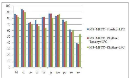
Bl, cl, co, di, hi, ja, me, po, re and ro in Table 3, 4 and 5 represent to blues, classical, country, disco, hiphop, jazz, metal, pop, reggae, and rock genre. From Table 3, it can be seen that blues genre has 87 instances that are correctly classified as their genre, 7 instances that are misclassified as country genre, 1 instance that is misclassified as disco genre, 2 instances that are misclassified as metal genre, 2 instances that are misclassified as reggae genre and 1 instance that is misclassified as rock genre. The best genre is classical with 95 instances that are correctly classified to their genre. The worst genre is rock with just 40 instances that are correctly classified to their genre.
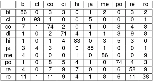
In Table 4 and 5 classical genre still become the best genre with 93 and 90 instances are correctly classified. The worst genre is rock with only 38 instances are correctly classified in Table 4. But, in Table 5, the number of correctly classified instance are increasing to 54 instances.
Table 3. Confusion Matrix of MS+MFCC+Tonality+LPC Features.
bl cl co di hi ja me po re ro
bl 87 0 7 1 0 0 2 0 2 1
cl 0 95 1 0 0 4 0 0 0 0
co 7 1 73 2 0 1 1 3 3 9
di 0 0 2 77 4 1 1 3 7 5
hi 1 0 1 5 82 0 3 5 3 0
ja 3 4 4 0 0 88 1 0 0 0
me 2 0 0 2 1 0 84 0 0 11
po 0 0 7 4 4 1 0 78 4 2
re 7 0 6 7 4 0 0 6 62 8
ro 12 1 10 8 4 0 9 6 10 40
Table 4. Confusion Matrix of All Feature Sets.
bl cl co di hi ja me po re ro
bl 86 0 3 3 0 1 2 0 3 2
cl 0 93 1 0 0 5 0 0 0 1
co 7 1 74 2 0 1 0 3 4 8
di 1 0 2 71 4 1 1 3 9 8
hi 1 0 1 4 83 0 3 5 3 0
ja 3 4 3 0 0 88 1 0 0 1
me 4 0 0 0 1 0 86 0 0 9
po 1 0 8 5 4 1 0 74 4 3
re 4 0 7 9 7 0 0 6 58 9
ro 11 1 11 9 4 1 8 6 11 38
Table 5. Confusion Matrix of MS+MFCC+Rhythm+LPC Features.
bl cl co di hi ja me po re ro
bl 83 0 6 1 0 1 4 0 1 4
cl 0 90 0 0 0 8 0 0 0 2
co 8 0 71 3 0 4 0 3 3 8
di 1 0 3 68 7 1 2 4 9 5
hi 5 0 2 13 65 0 2 4 8 1
ja 4 4 6 0 0 81 1 1 0 3
me 4 0 0 3 1 0 87 0 0 5
po 0 0 6 4 6 1 0 75 4 4
re 6 0 8 8 8 0 0 3 60 7
ro 10 0 10 4 2 2 10 3 5 54
Figure 3. Accuracy comparison of the three different feature combinations for each genre.
5. Concluding Remarks
The experiments of automatic musical genre classification have been done successfully using three SVM kernels toward different combination of audio feature set. The kernels are poly-nomial, radial basis function (RBF) and sigmoid. The audio feature sets used are musical surface, MFCC, rhythm, tonality and LPC. There are 31 possible combination of the feature sets. With the implementation of the three kernels, 93 experiments are done in this research. The result shows that the most appropriate kernel for automatic musical genre classification is polynomial kernel. While the best combination of audio features is the combination of musical surface, MFFC, tonality and LPC. The combination achieves classification accuracy of 76.6 %. This result is comparable to human performance in classifying music into a genre.
For future research, several things have to be considered. These include the usage of more varied genre to classify music and the development of an application for doing real time classification, i.e. detecting genre when a music piece is played on the radio, tv, mp3 player, and other electronic devices. Another important thing is conducting the research to label music into multiple genres. It is because, these days, a lot of music piece are composed based on the composition of two or more genres.
Acknowledgement
The authors would like to thank the Gunadarma Foundations for financial supports.
References
[1] G. Tzanetakis and P. Cook, “Musical genre classication of audio signals,” in IEEE Trans. Speech Audio Process, vol. 10, no. 5, July 2002, pp. 293–302.
[2] G. Tzanetakis, G. Essl, and P. Cook, “Automatic music genre classification of audio signals,” inProc. ISMIR, 2001.
[3] M. F. McKinney and J. Breebaart,Features for Audio and Music Classification, Philips Re-search Laboratories, Eindhoven, The Netherlands, 2003.
[4] P. D. Daniel McEnnis, Ichiro Fujinaga, “Jaudio: A feature extraction library,” inISMIR, 2005, Queen Mary, University of London.
[5] T. Li and G. Tzanetakis, “Factors in automatic musical genre classification of audio signals,” inIEEE Workshop on Applications of Signal Processing to Audio and Acoustics, New Paltz, NY, 19-22 Oct. 2003.
[6] E. G. Gutierrez, “Tonal description of music audio signals,” Ph.D. dissertation, Universitat Pompeu Fabra, 2006.
[8] “Gtzan genre collection.” [Online]. Available: http://marsyas.info/download/data sets/
[9] N. Scaringella, G. Zoia, and D. Mlynek, “Automatic genre classification of music content: a survey,”IEEE Signal Process. Mag., vol. 23, no. 2, pp. 133–141, Mar. 2006.
[10] F.Pachet and D. Cazaly, “A taxonomy of musical genres,” inProc. Content-Based Multimedia Information Access (RIAO), Paris, France, 2000.
[11] F. Pachet, J. Aucouturier, A. L. Burthe, A. Zils, and A. Beurive, “The cuidado music browser: an end-to-end electronic music distribution system,” inMultimedia Tools and Applications, 2004, Special Issue on the CBMI03 Conference, Rennes, France, 2003.
[12] D. Perrot and R. O. Gjerdigen, “Scanning the dial: An exploration of factors in the identifica-tion of musical style,” inProceedings of the 1999 Society for Music Perception and Cognition, 1999.
[13] K. Kosina, “Music genre recognition,” Master’s thesis, Hagenberg Technical University, Ha-genberg, Germany, June 2002.
[14] FFT Tutorial. ELE 436: Communication Systems, University of Rhode Island Department of Electrical and Computer Engineering. [Online]. Available: http://www.ele.uri.edu/∼hansenj/ projects/ele436/fft.pdf
[15] D. Mirovic, M. Zeppelzauer, and C. Breitender,Feature for Content-Based Audio Retrieval, Vienna University of Technology, 2010.
[16] S. McAdams, “Perspectives on the contribution of timbre to musical structure,” Computer Music Journal, vol. 23, pp. 85–102, 1999.
[17] B. Logan,Mel Frequency Cepstral Coefficients for Music Modelling, Cambridge Research Laboratory. Compaq Computer Corporation.
[18] P. R. Bhatt, “Audio coder using perceptual linear predictive coding,” Master’s thesis, B.E., C.U. Shah College of Engineering and Technology, India, 2006.
[19] “Support Vector Machines (SVM) introductory overview,” StatSoft Electronic Statistics Text-book, Accessed on January, 13 2014. [Online]. Available: http://www.statsoft.com/textbook/ support-vector-machines
[20] B. Santosa,Tutorial Support Vector Machine, Teknik Industri, ITS.
[21] B.-H. Kim,Support Vector Machine & Classification. using Weka, Biointelligence Lab. CSE, Seoul National University.
[22] F. Keller,Evaluation Connectionist and Statistical Language Processing, Computerlinguistik Universitaat des Saarlandes.
[23] S. V. Stehman, “Selecting and interpreting measures of thematic classification accuracy,” in Remote Sensing of Environment, vol. 62, no. 1, 1997, pp. 77–89, doi:10.1016/S0034-4257(97)00083-7.
[24] O. Lartillot, “Matlab toolbox for musical feature extraction from audio,” inInternational Con-ference on Digital Audio Effects, Bordeaux, 2007.
[25] D. McEnnis, C. McKay, and I. Fujinaga, “jaudio: Additions and improvements,” in ISMIR, 2006, Music Technology Area, McGill University, Montreal, Quebec.