Robust estimation of constrained covaria

(1)

Electronic copy available at: http://ssrn.com/abstract=1759977

Article

Reference

Robust Estimation of Constrained Covariance Matrices for

Confirmatory Factor Analysis

DUPUIS LOZERON, Elise, VICTORIA-FESER, Maria-Pia

Abstract

Confirmatory factor analysis (CFA) is a data anylsis procedure that is widely used in social and behavioral sciences in general and other applied sciences that deal with large quantities of data (variables). The classical estimator (and inference) procedures are based either on the maximum likelihood (ML) or generalized least squares (GLS) approaches which are known to be non robust to departures from the multivariate normal asumption underlying CFA. A natural robust estimator is obtained by first estimating the (mean and) covariance matrix of the manifest variables and then “plug-in” this statistic into the ML or GLS estimating equations. This twostage method however doesn’t fully take into account the covariance structure implied by the CFA model. An S -estimator for the parameters of the CFA model that is computed directly from the data is proposed instead and the corresponding estimating equations and an iterative procedure derived. It is also shown that the two estimators have different asymptotic properties. A simulation study compares the finite sample properties of both estimators showing that the proposed direct estimator is more stable (smaller MSE) than the two-stage estimator.

DUPUIS LOZERON, Elise, VICTORIA-FESER, Maria-Pia. Robust Estimation of Constrained

Covariance Matrices for Confirmatory Factor Analysis. Computational Statistics and Data

Analysis, 2010

Available at:

Disclaimer: layout of this document may differ from the published version.

[ Downloaded 11/02/2011 at 15:06:10 ]

(2)

Robust Estimation of Constrained Covariance Matrices for

Confirmatory Factor Analysis

E. Dupuis Lozerona_{, M.P. Victoria-Feser}a

a_{HEC,University of Geneva,1211 Geneva, Switzerland}

Abstract

Confirmatory factor analysis (CFA) is a data anylsis procedure that is widely used in social and behavioral sciences in general and other applied sciences that deal with large quantities of data (variables). The classical estimator (and inference) procedures are based either on the maximum likelihood (ML) or generalized least squares (GLS) approaches which are known to be non robust to departures from the multivariate normal asumption underlying CFA. A natural robust estimator is obtained by first estimating the (mean and) covariance matrix of the manifest variables and then “plug-in” this statistic into the ML or GLS estimating equations. This two-stage method however doesn’t fully take into account the covariance structure implied by the CFA model. An S-estimator for the parameters of the CFA model that is computed directly from the data is proposed instead and the corresponding estimating equations and an iterative procedure derived. It is also shown that the two estimators have different asymptotic properties. A simulation study compares the finite sample properties of both estimators showing that the proposed direct estimator is more stable (smaller MSE) than the two-stage estimator.

Key words: S-estimator, asymptotic efficiency, generalized least squares, structural equations modeling, two-stage estimation

1. Introduction

Factor analysis (FA) is an old technique that is widely used not only as a data reduction tech-nique, but also for the construction of measurement scales as is done for example in psychology. It is also used for the analysis of data in social and behavioral sciences in general and other applied sciences that deal with large quantities of data (variables). Given a vector of observed (manifest) variablesX =(X1, ...,Xp)T ∈ Rp with mean vectorµ =(µ1, ..., µp)T and covariance matrixΣ, the FA model states that

X₋µ=Γf+ǫ,

where f = (f1, ...,fk)T is the vector containingk < p factors, Γis the p×kmatrix of factor loadings and ǫ is the error term. It is also assumed thatcov(f,ǫ) = 0, E[f] = 0k, E[ǫ] = 0p,E[f fT] = Φk×k,E[ǫǫT] = Ψp×p andΨ = diag{ψ₁2, ..., ψ2p}, where theψ2j are the so-called

Email addresses:Elise.Dupuis@unige.ch(E. Dupuis Lozeron),Maria-Pia.VictoriaFeser@unige.ch (M.P. Victoria-Feser)

(3)

uniqueness. Moreover, sinceE[(X−µ)(X−µ)T]=E[(Γf+ǫ)(Γf+ǫ)T], the FA model is also often presented as

Σ=ΓΦΓT+Ψ. (1)

The loadings matrixΓ, containing sayqunknown factor loadingsγ1, . . . , γq, can be either full for so-called exploratory FA (i.e. q=p_·k) or constrained (typically some loadings are set to 0) for so-called confirmatory FA (i.e. q < p_·k). In what follows, we will assume that the factors are normal and independent, i.e.Φ=Ip, but this hypothesis could be relaxed.

Given a sample ofnobservations on thepmanifest variables, with classical FA,µis estimated by the sample mean ¯xandΣis estimated by the sample covariance matrixS. Estimates forΨand

Γare then found by maximum likelihood estimator (MLE) algorithm asSis supposed to have a Whishart distribution ifXis multivariate normal (see J¨oreskog, 1967). However, it is well known that the sample mean and covariance are not robust estimators of their corresponding population parameters, in that small departures from the normality assumption on the manifest variables can seriously bias the FA parameter estimates (see e.g. Yuan and Bentler, 1998, 2001; Pison et al., 2003). This is also true for alternative estimators to the MLE, such as generalized least squares (GLS) methods (see Browne, 1984).

To avoid potential biases due to the violation of the normality assumption, one can simply estimate the mean and covariance of the manifest variables in a robust fashion and “plug in” the estimates in a classical objective functionL(to be minimized), such as the one for the MLE based on the Whishart distribution, i.e.,

LML(θ)=log|Σ(θ)|+tr[SΣ(θ)−1]−log|S| −p, (2)

or the one for the GLS

LGLS(θ)=( ˆσ−σ(θ))TW( ˆσ−σ(θ)), (3) whereWis some weight matrix,θis the vector of parameters of interest (theγj andψ2j),Σ(θ) depends onθthrough (1) andσ(θ)=vec(Σ(θ)) and ˆσ=vec(S), where the operator vec(.) stacks the columns of a matrix on top of each other. There are different possibilities for the choice of W, the one leading to the most efficient estimator ofθbeing the asymptotic covariance matrix of ˆσ. In practice, this quantity is replaced by a suitable estimate which possibly depends on the unknown parametersθ. This type of procedure that has been formalized in e.g. Yuan and Bentler (1998) and Pison et al. (2003), provides consistent estimators of the FA model’s parameters. An alternative approach for robust estimation of FA models is also given in Croux et al. (2003).

(4)

2. Robust estimators for FA

2.1. Two-stage estimator

To estimateµandΣ, we use anS-estimator with a high breakdown point. Very generally, an S-estimator of multivariate location and scale is defined as the solution for µandΣ that minimizes the determinant ofΣ, i.e.|Σ|, subject to

1

n n

X

i=1

ρ

q

(xi−µ)TΣ−1(xi−µ)

!

=1

n n

X

i=1

ρ(di)=b0, (4)

where ρis a symmetric, continuously differentiable function, with ρ(0) = 0 andρis strictly increasing on [0,c] and constant on [c,_∞] andcis such that E_Φ[ρ]/ρ(c) = ǫ∗ _where_Φ_{is the}

standard normal andǫ∗_{is the chosen breakdown point (see Rousseeuw and Yohai, 1984) .}_b₀_is

a parameter chosen to determine the breakdown point by means ofb0=ǫ∗maxdρ(d).

Forρ, we use the biweightρ-function of Tukey. Hence, the biweightS-estimator (BS) is defined by the minimum of|Σ|subject to (4), with

ρ(d;c)=

      

d2_/2

−d4_/(2_c2₎₊_d6_/(6_c4_), ₀

≤d_≤c

c2/6. d>c (5)

Estimating equations for theBS-estimator are

µ = Pn 1 i=1u(di;c)

n

X

i=1

u(di;c)xi, (6)

Σ = _Pn p i=1u(di;c)d2i

n

X

i=1

u(di;c) (xi−µ) (xi−µ)T,

with weights

u(d;c)= 1

d

∂

∂dρ(d;c)=

      

1−(d/c)22_, ₀

≤d_≤c

0. d>c

The BS-estimator ofΣcan then be used to replaceSor ˆσin the objective functions (2) or (3); this defines the two-stage estimator (MLE or GLS).

2.2. Direct estimator

The FA model implies that the data have been generated by a multivariate normal distribution with constrained covariance matrix according to (1). For this type of problems, one can use the results of Copt and Victoria-Feser (2006) who have developed such an estimator for mixed linear models.

In Appendix A, we derive estimating equations for the FA parameters directly from the ob-jective function of theS-estimator, using the Lagrangian of the minimization of|Σ|subject to (4) given by

L=log|Σ|+λ

      

1

n n

X

i=1

ρ(di;c)−b0

      

(5)

LetP0=

h

ψ2 1, ..., ψ

2

p

iT

andG0=

h

γ1, ..., γq

iT

, an iterative system for theγjandψjis given by

P(₀t+1) = p

n

      

1

n n

X

i=1

u(di;c)(t)d2(_i t)

      

−1

C−1(t)D(t),

G(₀t+1) = p

n

      

1

n n

X

i=1

u(di;c)(t)d2(_i t)

      

−1

M−1(t)N(t),

with the matricesC,D,MandNgiven in respectively (26), (27), (29) and (30). Note thatµis calculated at each step with equation (6) andΣfromG0andP0.

For the starting point of this iterative procedure, one can perform a confirmatory FA based on a robust “plug-in” covariance matrix that is fast to compute. Our choice goes to the orthogo-nalized Gnanadesikan-Kettering (OGK) proposed by Maronna and Zamar (2002). Alternatively, for an even faster solution, one can perform an exploratory FA (on e.g. the OGK) and set the resulting loadings (γi j) that are constrained (e.g. to zero) to the constrained value (e.g. zero). We sucessfully implemented this last alternative and used it for the simulations. The resulting algorithm is as follows

1. Computeµstart=µOGKandΣOGK.

2. ComputeΨstartandΓstartby means of an exploratory factor analysis based onΣOGK. Re-place the fixedγi jinΓstartby their value (e.g. zero).

3. ComputeΣstart=ΓstartΓTstart+Ψstart. 4. Compute the Mahalanobis distanced(1)_i =

q

(xi−µstart)TΣ−

1

start(xi−µstart). 5. Compute the different weightsu(d(1)_i ;c).

6. Compute the mean vector

µ(1)=

Pn i=1u(d

(1)

i ;c)xi

Pn i=1u(d

(1)

i ;c) .

7. Compute the vector of loadingsG0and uniquenessP0

G(1)₀ = p

n

      

1

n n

X

i=1

u(di;c)(1)d2(1)_i

      

−1

M−1(1)N(1),

P(1)₀ = p

n

      

1

n n

X

i=1

u(di;c)(1)d

2(1)

i

      

−1

C−1(1)D(1).

8. UsingP(1)₀ andG(1)₀ computeΣ(1).

9. Use a convergence criterion; if the conditions of convergence are met stop, otherwise start again from (4) and putµ_start=µ(1)_and_Σ

start=Σ(1). Repeat the procedure until convergence is reached.

3. Inference for the direct and two-stage estimators

3.1. Direct estimator

To compute the asymptotic covarianceVG0 of the loadings estimator ˆG0 andVP0 of the

(6)

together with the delta-method. The asymptotic covariance of √nvec( ˆΣ) is

V_Σ=e3(Ip2+K_p,p)Σ⊗Σ+e4vec(Σ)vec(Σ)T, (8)

where⊗denotes the Kronecker product andKp,p is a (p2×p2)-block matrix with (i,j)-block being ap_×pmatrix with 1 at entry (j,i) and 0 elsewhere. The constantse3ande4are given by

e3 =

p(p+2)E_Φ[ψ2₍_d_;_c₎_d2_]

E_Φ2_ψ_′

(d;c)d2₊₍_p₊_1)ψ(_d_;_c₎_d, (9)

e4 = −

2

pe3+

4E_Φ[ρ(d;c)−b0]2

E2_Φ[ψ(d;c)d] . (10)

withpthe dimension ofΣ,ψ(d;c)=(∂/∂d)ρ(d;c). The expectations are taken at the standard-ized p-variate normal distributionΦ. The values ofe3ande4 can be obtained by Monte-Carlo

simulation.

The minimization of (7) provides the solutions ˆG0 and ˆP0 and ˆΣis actually a function of

the latter. To find the (asymptotic) variance of ˆG0 and ˆP0 one can use the delta-method. Let

D_Γ =_∂_G∂T

0

vecΣ(G0,P0)andDΨ=∂∂PT₀vecΣ(G0,P0)

, withΣ(G0,P0)=Γ(G0)ΓT(G0)+Ψ(P0).

We then have

VG0= DΓ

T_D

Γ−

1

D_ΓTV_ΣD_Γ D_ΓTD_Γ−1_, ₍₁₁₎

and

VP0= DΨ

T_D

Ψ−

1

D_ΨTV_ΣD_Ψ D_ΨTD_Ψ−1_.

(12)

ForD_Γ, we have

D_Γ=

"

∂ ∂γ1

vec(Σ) . . . ∂ ∂γq

vec(Σ)

#

=

"

∂ ∂γ1

vec(ΓΓT) . . . ∂ ∂γq

vec(ΓΓT)

#

,

=

"

vec( ∂ ∂γ1ΓΓ

T

) . . . vec( ∂ ∂γqΓΓ

T )

#

,

=

"

vec ( ∂ ∂γ1Γ

)ΓT

+vecΓ( ∂

∂γ1Γ

T ) _{. . .}

vec ( ∂ ∂γqΓ

)ΓT

+vecΓ( ∂

∂γqΓ T

) #

.

Because vec(AB)=(Ip⊗A)vec(B)=(BT⊗Im)vec(A) whereAis anm×nmatrix andBis an n_×qmatrix (see e.g. Magnus and Neudecker, 1988), we obtain that

D_Γ =

"

Ip⊗( ∂ γ1

)Γ

!

vec(ΓT)+ (∂ γ1

ΓT)T⊗Ip

!

vec(Γ) . . .

Ip⊗( ∂ γq

)Γ

!

vec(ΓT)+ (∂ γq

ΓT)T⊗Ip

!

vec(Γ)

#

. (13)

3.2. Two-stage estimator

The two-stage estimator ˆθis the result of the minimization of (3), i.e. the solution inθof

∂σ(θ)

(7)

The asymptotic variance of ˆθis equal to (see e.g. Yuan and Bentler, 1998)

Ω=A−1ΠA−1, (15)

with A = ∂_∂σ_θ(Tθ)

T

W∂_∂σ_θ(Tθ), Π =

_∂_σ₍_θ₎

∂θT

T

WV_ΣW∂_∂σ_θ(Tθ) andVΣ being the asymptotic variance

of √nσˆ = √nvec( ˆΣ). (14) actually defines a class of GLS estimators within which the most efficient (and equivalent to the MLE) is obtained whenW=V−_Σ1, which is replaced in practice by a sample estimate ofV_Σ. Hence for the MLE, (15) simplifies to

Ω= ∂σ(θ)

∂θT

T

V−_Σ1∂σ(θ) ∂θT

!−1

. (16)

Whenθcontains only the loadings, (16) can be written as

VG0 = DΓ

T

V−_Σ1D_Γ−1_,

(17)

withV_Σgiven in (8). One can see that (11) and (17) are equal ifD_Γis a square matrix, but not in the other cases. It is however not clear which of the asymptotic covariance matrices is smaller, and hence which of the two-stage or direct estimators is the most efficient.

4. Simulation study

The aim of the simulation study is to compare the (direct)CBS estimator with respectively the classical two-stage estimator (i.e based on the Pearson correlations) and the two-stage es-timator using the robust BS-estimator as covariance matrix estimator, under different kinds of models and data contamination. For both robust estimators, the breakdown point ǫ∗ is set to 50%. For the classical and robust two-stage estimators we use the software Mplus, whereas we use the statistical package R (R Development Core Team, 2008) for the (direct)CBS, with the

OGK estimator as a starting point as well as for computing theBS-estimator. We try both the MLE and the GLS objective function in Mplus for the classical and robust two-stage estimators, but the latter doesn’t seem to be reliable in relatively small samples (n =40 , p =20) as will be shown below with Figure 1. Therefore, we will finally compare three estimators, the classical and robust two-stage estimators (with, respectively, the Pearson or theBS covariance estimates) with the ML objective function (ML(P) andML(BS)) and the (direct)CBS.

The data are generated from two different models, a model with a relatively small number of manifest variables (p=6) for which we simulate relatively large samples (n=100) and a model with a relatively large number of manifest variables (p = 20) for which we simulate relatively small samples (n=40). In both models, we set the number of latent variables to 2, and for each of them, two sets of values forΓwere chosen in order to create a strong and weak signal to noise ratio. The values of the parameters for all models can be found in Appendix B. For the model withp=6, the number of loadings different from 0 (q) is equal topand for the other model we choose 2 different values forq, namelyq=p=20 andq=26.

The contamination consists in generating (1−ǫ)% of the data from a multivariate normal distribution with parameters given by the model andǫ% of the data from a multivariate normal distribution with one third of the loadings different from 0 that are multiplied by 10. Different amounts of contamination are chosen, but we present here only theǫ₌5% case.

(8)

and (17) with the true values of the parameters. With our chosen set of parameters, whenq=p

the efficiency is approximately one but whenq > pthe two-stage estimator is asymptotically more efficient (see values in Appendix B).

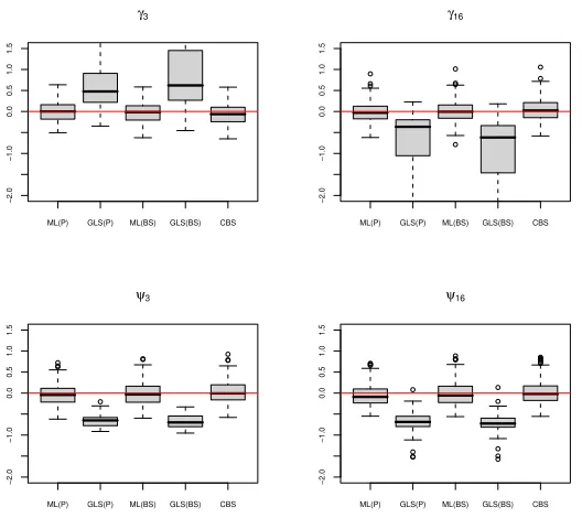
In Figure 1 are presented the bias distributions of the loadings’ and uniqueness’ estimators for the model withn=40 (q=p=20) and a high signal to noise ratio, without data contamination. The estimators are the two-stage estimators using respectively the MLor theGLS objective functions, with the Pearson correlations or theBSestimator, as well as the directCBSestimation. As mentioned previously, it seems that using theGLS objective function produces unreliable results, while the other estimators (ML(P),ML(BS) andCBS) behave well (unbiased) and in the same manner (same variances).

ML(P) GLS(P) ML(BS) GLS(BS) CBS

−2.0

−1.0

0.0

0.5

1.0

1.5

γ3

−2.0

−1.0

0.0

0.5

1.0

1.5

γ16

−2.0

−1.0

0.0

0.5

1.0

1.5

ψ3

−2.0

−1.0

0.0

0.5

1.0

1.5

ψ16

Figure 1: Bias distribution of the loadings’ and uniqueness’ estimators for the model withn=40, no contamination and a high signal to noise ratio

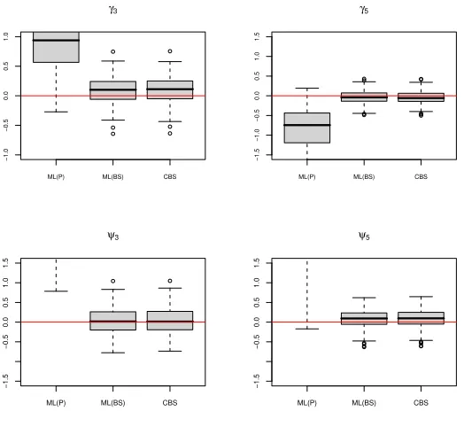
When there is data contamination, not surprisingly the simulations show that the two-stage estimator based on the Pearson’s covariance matrix is biased, whereas this is not the case with theCBS and the two-stage estimator based on theBS (see Figure 2).

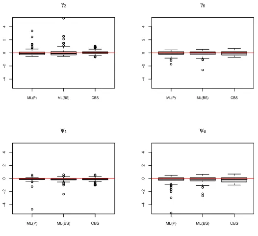
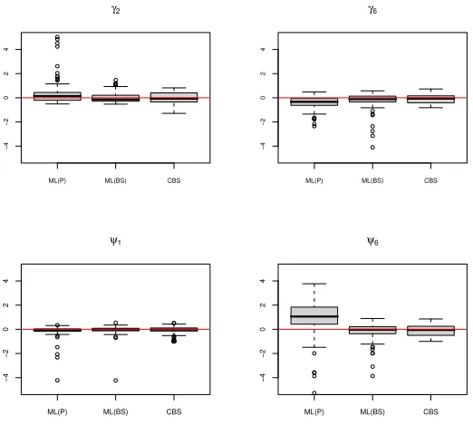
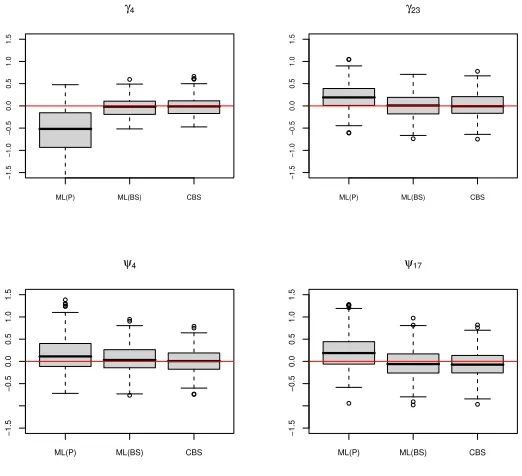
Overall, the two robust estimators (ML(BS) andCBS) seem to be pretty similar in terms of bias and variance. However, in one case (n = 100,p = 6 and low signal to noise ratio) the two-stage estimator produces extreme estimates for the loadings and negative ones for the uniqueness, as can be seen in Figures 3 and 4. The Mean Square Error of the two-stage estimator is really larger than that of theCBS in that case (see Table 1). This could be due to the fact that the two-stage estimator needs the estimation of a full covariance matrix.

(9)

ML(P) ML(BS) CBS

−1.0

−0.5

0.0

0.5

1.0

γ3

ML(P) ML(BS) CBS

−1.5

−1.0

−0.5

0.0

0.5

1.0

1.5

γ5

ML(P) ML(BS) CBS

−1.5

−0.5

0.0

0.5

1.0

1.5

ψ3

ML(P) ML(BS) CBS

−1.5

−0.5

0.0

0.5

1.0

1.5

ψ5

Figure 2: Bias distribution of the loadings’ and uniqueness’ estimators for the model withp=6, data contamination and a high signal to noise ratio

of the two-stage estimator, with finite samples, theCBS doesn’t seem to be more variable than the two-stage estimator with or without data contamination, as illustrated in Figure 5. This might be explained by the fact that since p is large relative ton, theBS estimator can be very (computationally) unstable so that its finite sample variance is (artificially) increased. With the

CBS the number of parameters to estimate is smaller relative to the sample size, hence providing more (computationally) stable estimators.

(10)

ML(P) ML(BS) CBS

−4

−2

0

2

4

γ2

ML(P) ML(BS) CBS

−4

−2

0

2

4

γ6

ML(P) ML(BS) CBS

−4

−2

0

2

4

ψ1

ML(P) ML(BS) CBS

−4

−2

0

2

4

ψ6

Figure 3: Bias distribution of the loadings’ and uniqueness’ estimators for the model withp=6 without data contami-nation and with a low signal to noise ratio

Table 1: MSE×100 for the model withp=6, low signal to noise ratio

ǫa ₌_0% _ǫ₌_5%

ML(P) ML(BS) CBS ML(P) ML(BS) CBS γ1 5.45 4.82 9.24 7.72 6.57 10.91

γ2 17.14 31.74 16.19 63.09 9.74 18.32

γ3 9.35 23.39 15.67 22.86 15.99 16.53

γ4 10.63 54.25 13.02 31.96 35.76 13.88

γ5 1.24 1.31 3.60 1.35 1.72 4.16

γ6 6.86 8.78 9.82 44.43 28.16 12.09

ψ1 13.45 5.53 9.79 16.52 10.93 10.97

ψ2 174.50 692.83 26.61 1536.86 30.74 28.27

ψ3 56.35 275.53 25.17 244.39 110.70 26.43

ψ4 62.63 4658.36 30.62 1338.24 1013.10 34.91

ψ5 1.51 1.76 5.40 1.43 2.27 5.95

ψ6 30.47 69.43 23.58 1348.62 445.21 26.20

(11)

ML(P) ML(BS) CBS

−4

−2

0

2

4

γ2

ML(P) ML(BS) CBS

−4

−2

0

2

4

γ6

ML(P) ML(BS) CBS

−4

−2

0

2

4

ψ1

ML(P) ML(BS) CBS

−4

−2

0

2

4

ψ6

(12)

ML(P) ML(BS) CBS

−1.5

−1.0

−0.5

0.0

0.5

1.0

1.5

γ4

ML(P) ML(BS) CBS

−1.5

−1.0

−0.5

0.0

0.5

1.0

1.5

γ23

ML(P) ML(BS) CBS

−1.5

−0.5

0.0

0.5

1.0

1.5

ψ4

ML(P) ML(BS) CBS

−1.5

−0.5

0.0

0.5

1.0

1.5

ψ17

(13)

5. Conclusion

To estimate in a robust fashion the parameters of a FA model, one can choose between two strategies. One can compute a two-stage estimator by which a robust covariance matrix of the manifest variables is first computed and then used in the MLE or GLS estimating equations, possibly using a software, such as Mplus, available in the market. Alternatively, one can directly estimate the FA parameters (loadings and uniqueness) from a robust objective function such as the one of anS-estimator, in the same spirit as is done in Copt and Victoria-Feser (2006) for the mixed linear model. In this paper we derive the estimating equations (and an iterative procedure) for theS-estimator of the FA model, i.e. theCBS-estimator. The two estimators have different asymptotic properties, in that their asymptotic covariance matrix is not the same. With the models used in the simulation study, we found that the (trace of the) asymptotic covariance matrix of the two-stage estimator is even smaller. However, in finite samples, theCBS-estimator seems to be more stable than the two-stage estimator (smaller MSE).

Finally, the aim of this paper was to compare different approaches to robust estimation of FA models. A step further would be to evaluate the models using a goodness-of-fit type cri-terion or test statistic. A natural choice is a likelihood ratio type test on the covariance ma-trix (see e.g. Bartholomew and Knott, 1999) which compares the log-likelihood evaluated with

ˆ

Σ = Γ( ˆG0)ΓT( ˆG0)+Ψ( ˆP0) the constrained covariance matrix and that evaluated with the

(14)

A. Derivation of the estimating equations for the CBS-estimator

Using_∂θ∂

jlog|Σ|=tr

Σ−1∂θ∂Σj

and_∂θ∂

jΣ −1

=−Σ−1∂θ∂ΣjΣ −1

withθjany element ofθ, the vector of the FA parameters, as well as_∂γ∂

jΣ=

∂_Γ ∂γj

ΓT+Γ

∂_ΓT ∂γj

the partial derivatives of the Lagrangian (7) are then

∂

∂µL=−λ 1

n

Pn

i=1u(di;c)Σ−1(xi−µ)=0, (18) ∂

∂ψ2

jL=

tr[Σ−1Zj]−₂λ_nPni=1u(di;c)(xi−µ)TΣ−1ZjΣ−1(xi−µ)=0, (19)

withZj= _∂ψ∂2

jΣ= ∂ ∂ψ2

j

(ΓΓT +Ψ), and

∂ ∂γjL

=tr

Σ−1 ∂

∂γj

Γ

!

ΓT +Σ−1Γ ∂

∂γj

ΓT

!

−

λ 2n

n

X

i=1

u(di;c)(xi−µ)TΣ−1

_∂

∂γj

ΓΓT+Γ ∂

∂γj

ΓT

Σ−1(xi−µ)=0.

(20)

¿From (18) we get the estimating equation forµgiven in (6). Then, multiplying (19) byψ2_j and using the properties of the trace we get

tr[Σ−1Zjψ2j]− λ 2n

n

X

i=1

u(di;c)(xi−µ)TΣ−1Zjψ2jΣ−

1

(xi−µ)= 0,

r

X

j=1

tr[Σ−1Zjψ2j]− λ 2n

r

X

j=1

n

X

i=1

u(di;c)(xi−µ)TΣ−1Zjψ2jΣ−

1

(xi−µ)= 0,

tr[Σ−1

r

X

j=1

Zjψ2j]− λ 2n

n

X

i=1

u(di;c)(xi−µ)TΣ−1 r

X

j=1

Zjψ2jΣ−

1

(xi−µ)= 0,

tr[Σ−1Ψ]− λ

2n n

X

i=1

(15)

Similarly for (20) we get

Multiplying (21) by 2 and adding the result to (22) we obtain

2tr[Σ−1Ψ]+2tr[Σ−1ΓΓT]−λ

(16)

and

(23) and (24) are the estimating equations for the parametersγjandψj.

To define an iterative system, we need now to extractψjandγjfrom (23) and (24). First, we useΨ=Pr

which defines an iterative system for eachψ2

k,k=1, . . . ,r. Let

an expression for theψ2

jis given by

γjto reformulate the left hand side of (24) as

tr

so that

(17)

B. Parameter’s values for the simulations

B.1. First Model : n=100, p=6

We first choose the parameter’s valuesµ,ΓandΨso that the signal to noise ratio is high. They are

µ=[0,0,0,0,0,0]T, _Γ=

For a low signal to noise ratio case, we choose forµ,ΓandΨthe following values

(18)

The efficiency of theML(BS) relative to theCBSis 0.999.

(19)

are

For a low signal to noise ratio and 26 loadings different from zero, the values forµ,ΓandΨ

are

0.47 0.31

(20)

References

Bartholomew, D. J., Knott, M., 1999. Latent Variable Models and Factor Analysis. Kendall’s Library of Statistics 7. Arnold, London.

Browne, M. W., 1984. Asymptotically distribution-free methods for the analysis of covariance structures. British Journal of Mathematical and Statistical Psychology 37, 62–83.

Copt, S., Victoria-Feser, M.-P., 2006. High breakdown inference in the mixed linear model. Journal of the American Statistical Association 101, 292–300.

Croux, C., Filzmoser, P., Pison, G., Rousseeuw, P. J., 2003. Fitting multiplicative models by robust alternating regres-sions. Statistics and Computing 13, 23–36.

Heritier, S., Ronchetti, E., 1994. Robust bounded-influence tests in general parametric models. Journal of the American Statistical Association 89 (427), 897–904.

J ¨oreskog, K. G., 1967. Some contributions to maximum likelihood factor analysis. Psychometrika 32, 443–482. Lopuha¨a, H. P., 1989. On the relation between S-estimators and M-estimators of multivariatelocation and covariance.

The Annals of Statistics 17, 1662–1683.

Magnus, J. R., Neudecker, H., 1988. Matrix Differential Calculus with Applications in Statistics and Econometrics. John Wiley & Sons.

Maronna, R. A., Zamar, R. H., 2002. Robust estimates of location and dispersion for high-dimensional datasets. Techno-metrics 44, 307–317.

Pison, G., Rousseeuw, P. J., Filzmoser, P., Croux, C., 2003. Robust factor analysis. Journal of Multivariate Analysis 84 (1), 145–172.

R Development Core Team, 2008. R: A Language and Environment for Statistical Computing. R Foundation for Statis-tical Computing, Vienna, Austria, ISBN 3-900051-07-0.

URLhttp://www.R-project.org

Rousseeuw, P. J., Yohai, V. J., 1984. Robust regression by means of S-estimators. In: Franke, J. W., Hardle, Martin, R. D. (Eds.), Robust and Nonlinear Time Series Analysis. Springer-Verlag, New York, pp. 256–272.

Yuan, K.-H., Bentler, P. M., 1998. Robust mean and covariance structure analysis. British Journal of Mathematical and Statistical Psychology 51, 63–88.