Chapter II
THEORETICAL BACKGROUND
There are times when a company has to grow; this may comes as a result
of many occurrences, such as growing competitors, to boost income, necessity to
give selections to customers, etc. If a business is stagnant when a competitor
grows, soon the business will lose its customers to its competitor, which may offer
more varieties, or made cheaper product. So, a business has to grow, simply due
to the nature of the competitive environment that will not let it survive without
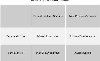
emerging. According to Philip Kotler, there are four ways for a company to grow.
Figure II.1
Kotler Growth Strategy Matrix
Present Products/Services New Products/Services
Present Markets Market Penetration Product Development
This matrix allows businessman to consider ways to grow the business via
existing and/or new products, in existing and/or new markets (there are four
possible product/market combinations). This matrix consist of four strategies:
1. Market Penetration (existing market, existing product)
Occurs when a company enters a market with current products. The best
way to achieve this is by gaining competitors’ customers (part of their
market share). Other ways include attracting non-users of their product or
convincing current clients to use more of their product/service, with
advertising or other promotions.
2. Product Development (existing market, new product)
A company with a market for its current product might embark on a
strategy of developing other products catering to the same market. For
example, McDonalds is always within the fast-food industry, but
frequently markets new burgers. Frequently, when a firm creates new
products, it can gain new customers for these products. This is the strategy
which Marga Agung want to pursue, same market but with new product
which is furniture.
3. Market Development (new market, existing product)
An established product in the marketplace can be targeted to a different
customer segment as well as non-buying customers in currently targeted
market, as a strategy to earn more revenue for the company. Exporting the
product, or marketing it in a new region is examples of market
4. Diversification (new market, new product)
Diversification is a form of growth marketing strategy for a company. It
seeks to increase profitability through greater sales volume obtained from
new products and new markets. Virgin Cola, Virgin Megastores, Virgin
Airlines, Virgin Telecommunications are examples of new products
created by the Virgin Group of UK, to leverage the Virgin brand. This
resulted in the company entering new markets where it had no presence
before.
II.1. Business Plan
Business plan is a very important tool for a businessman or a decision
maker in a company to make sure whether the ongoing and upcoming business
activity is on track as it has been planned before. (Rangkuti, 2005) Business
activity can be creating a new business, developing the existing business (merger,
raise the fund, adapting new technology, opening new branch office, etc), or
acquisition of a business.
The purpose of business plan is to minimize the risk associated with a new
business and maximize the chances of success through research and maximize the
chance for success through research and planning. (Subagyo, 2008) Businessman
also use business plan to searching fund from third party, such as bank, investor,
etc.
There are four important elements in a business plan, which are:
2. Marketing plan
3. Financial management plan
4. Operational management plan
II.2. Investment Analysis II.2.1. Depreciation
Pujawan (1995) says that depreciation and tax are two important factors
that must be considered in feasibility study. Although depreciation is not a cash
flow, but its amount and its time will influence tax that must be paid by the
company. Tax is a cash flow. For that reason, tax must be considered as tools cost,
material, energy, worker, etc. A good knowledge about depreciation and tax
system will help in make a decision related to investment.
Depreciation is value reduction of a property or an asset because of time
and usage. Depreciation of a property (asset) usually caused by these one or more
factors:
a. Physical damage because the usage its tool or property.
b. Newer and bigger production need or service.
c. Decreasing production need or service.
d. The property becomes obsolete because of technology development.
e. The invention of facilities that can earn more products with lower cost and
better safety level.
Not all properties can be depreciated. There are several qualifications that
a. Must be used in business necessity or to earn income.
b. Economic life is countable.
c. Economic life more than a year.
d. Must be something that used, something that become obsolete, or
something that its value decreased because of scientific reasons.
There are many methods that can be used to determine yearly depreciation
of an asset. From all the methods, the most popular are:
a. Straight Line method or SL
b. Sum of Year Digit method or SOYD
c. Declining Balance method or DB
d. Sinking Fund method or SF
II.2.1.1. Straight Line Method or SL
This method is based on assumption that the decreasing of an asset
linearly (proportionally) to time or age of that asset. This method is commonly
used because it is easy and simple. The formula of Straight Line method:
Depreciation = (Cost - Residual value) / Useful life
Dt PS
N
Information:
Dt = depreciation at t year
P = purchase price of asset
S = salvage value
II.2.1.2. Sum of Year Digit Method or SOYD
This method is designed to charge bigger depreciation at the beginning
year and smaller for the next years. This means Sum of Year Digit charge
depreciation faster that Straight Line method. Accelerated depreciation method in
which the amounts recognized in the early periods of an asset's useful life are
greater than those recognized in the later periods. The SYD is found by estimating
an asset's useful life in years, assigning consecutive numbers to each year, and
totaling these numbers. For n years, the short-cut formula for summing these
numbers is SYD = n(n + 1)/2. The yearly depreciation is then calculated by
multiplying the total depreciable amount for the asset's useful life by a fraction
whose numerator is the remaining useful life and whose denominator is the SYD.
Thus annual depreciation equals
II.2.1.3. Declining Balance Method or DB
This method is similar to Sum of year Digit. This method used if asset age
more than 3 years. The depreciation value of the certain year determined by
multiplies fixed percentage of asset value in the end of the previous year.
DtdBVt1
Information:
d = determined depreciation
BVt-1 = asset value at the end of the previous year
F = residue value
P= invest value
T = economic life
II.2.1.4. Sinking Fund Method or SF
This method use assumption that the depreciation of the next year is faster
than previous year. The formula of Sinking method:
Dt(PS)(A/F,i%,N)(F/P,i%,t1)
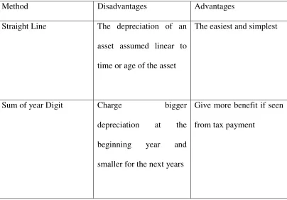
Table II.1
The advantages and disadvantages of the methods
Method Disadvantages Advantages
Straight Line The depreciation of an
asset assumed linear to
time or age of the asset
The easiest and simplest
Sum of year Digit Charge bigger
depreciation at the
beginning year and
smaller for the next years
Give more benefit if seen
Declining Balance Can be used if the asset
age is more than 3 years,
is not suitable for short
age asset. Depreciation
load is bigger at the
beginning and decrease at
the next years, but the
depreciation is faster than
sum of year digit.
Gives more benefits if
seen from the payment of
income tax. This method
has residue value from an
asset will be reached at
the end of the asset life.
Sinking Fund Is not give benefit if seen
from the payment of
income tax.
Depreciation load less at
the beginning and greater
at the next years. This
method is good if in the
calculation, interest is
considered.
Source Pujawan, 2003
II.2.2. Minimum Attractive Rate of Return (MARR)
Pujawan (1995) said interest rate that used as a basic standard in
evaluating and comparing many alternatives named MARR. MARR is the
minimum value from rate of return or acceptable interest by investor. With rate of
return smaller than MARR so that investment is not economically good and
For feasibility study, interest rate used is manufacture’s MARR. Usually
each manufacture determines their own MARR standard to consider their
investments. MARR calculation formula is:
MARR = ir + if + (ir) (if)
Where, ir = interest rate / year and if = inflation rate
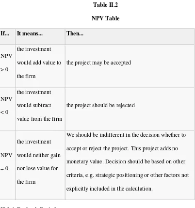
II.2.3. Net Present Value (NPV)
As the flaws in the payback method were recognized, people begin to
search for methods of evaluating projects that would recognize that a dollar
receive immediately is preferable to a dollar received at some future date. This led
to the development of discounted cash flow (DCF) techniques to take account of
the time value of money. One such DCF technique is called the net present value
method. TO implement this approach, find the present value of the expected net
cash flows of an investment, discounted at an appropriate percentage rate, and
subtract from it the initial outlay of the project. If its net present value of the
project is positive, the project should be accepted; if negative it should be
rejected. Of two projects are mutually exclusive, the one with the higher net
present value should be chosen.
The equation for the net present value (NPV) is
NPV= R1
Here R1, R2, and so forth represent the annual receipts, or net cash flows; k is the
riskiness of the project, the level of interest rates in the economy, and several
the project may be accepted
NPV
< 0
the investment
would subtract
value from the firm
the project should be rejected
NPV
We should be indifferent in the decision whether to
accept or reject the project. This project adds no
monetary value. Decision should be based on other
criteria, e.g. strategic positioning or other factors not
explicitly included in the calculation.
II.2.4. Payback Period
The Payback period is defined as the number of years it takes a firm to
Payback period method generally use only for smaller replacement projects or as a
risk indicator in larger projects. Some features of the payback, which indicate both
its strengths and weaknesses, are listed below:
1. Ease of Calculation. The payback is easy to calculate and apply. This was
an important consideration in the pre-computer days.
2. Ignores Returns Beyond Payback Period. One glaring weakness of the
payback method is that it ignores returns beyond the payback period.
Ignoring returns in the distant future means that payback penalizes
long-term projects.
3. Ignores Time Value of Money. The timing of cash flows is obviously
important, yet the payback method ignores the time value of money.
II.2.5.Break Even Point (BEP)
The Break-even Point is, in general, the point at which the gains equal the
losses. A break-even point defines when an investment will generate a positive
return. The point where sales or revenues equal expenses. Or also the point where
total costs equal total revenues. There is no profit made or loss incurred at the
break-even point. This is important for anyone that manages a business, since the
break-even point is the lower limit of profit when prices are set and margins are
determined.
Achieving Break-even today does not return the losses occurred in the
past. Also it does not build up a reserve for future losses. And finally it does not
Break-even analysis is a useful tool to study the relationship between fixed
costs, variable costs and returns. The Break-even Point defines when an
investment will generate a positive return. It can be viewed graphically or with
simple mathematics. Break-even analysis calculates the volume of production at a
given price necessary to cover all costs. Break-even price analysis calculates the
price necessary at a given level of production to cover all costs. To explain how
break-even analysis works, it is necessary to define the cost items.
Fixed costs, which are incurred after the decision to enter into a business
activity is made, are not directly related to the level of production. Fixed costs
include, but are not limited to, depreciation on equipment, interest costs, taxes and
general overhead expenses. Total fixed costs are the sum of the fixed costs.
Variable costs change in direct relation to volume of output. They may
include cost of goods sold or production expenses, such as labor and electricity
costs, feed, fuel, veterinary, irrigation and other expenses directly related to the
production of a commodity or investment in a capital asset. Total variable costs
(TVC) are the sum of the variable costs for the specified level of production or
output. Average variable costs are the variable costs per unit of output or of TVC
divided by unit of output.
The Break-even Point analysis must not be mistaken for the Payback
Period the time it takes to recover an investment.
where:
BEP = break-even point (units of production)
TFC = total fixed costs,
VCUP = variable costs per unit of production,
SUP = selling price per unit of production.
II.2.6. Economical Life
The measurement of an economical life of an asset is used to determine
when that certain asset needs to be replaced. Indeed, the replacement will be done
if it is economically better than using the old asset (defender).
The economical life of an asset is a point of time period when the total
annual cost occurring is minimum. The total annual cost consists of annual
operation cost and maintenance cost. Annual operation and maintenance cost
usually increase as the usage time of the equipment is longer. Whereas the annual
cost from investment cost will decrease the longer the usage of the equipment.
Due to the replacement analysis will compare defender and challenger in
the base of its economical life, thus prior to comparing, it is necessary to be aware
of the calculation of economical life. This calculation will be easily done if the
cash flow can be predicted with high certainty. This analysis will only engage the
cost of annual equivalent in the end of every year as long as the age of that certain
equipment. Scientifically, the annual equivalent cost will decrease with the
increasing usage of an asset. This decrease will only occur for a certain usage
II.2.7. Inflation
Basically, inflation is defined as a time when the cost of goods, services,
or other general production factors increase. The inflation will make the buying
capability of money decrease from time to time. (Pujawan, 2004)
Pujawan (2004) mentions that with the occur of inflation, it will make the
present worth of money will be less in the future. In its correlation with financial
analysis, there are several things that can be done concerning inflation and
deflation, such as:
Convert all cash flow to present worth of money to eliminate the effect of
inflation, then use regular interest rate (interest rate without inflation effect
in interest formula). This method is more suitable for analysis before taxes
because all of the components of cash flow is inflated in the same rate.
State future value as present value and use interest rate that include
inflation effect. Interest rate that has considered inflation effect is called
inflated interest rate or combination inflation interest rate.
Pujawan (2004) mentions, if ifis the interest rate after inflation that should
be obtained by an investor from its investment that needs initial cost as much as P
and if is the inflation rate, therefore the future value from the investment after n
year is:
F = P (1+if)N
Where ic is the combination of inflation interest rate that shows the
minimum rate required for an acceptable investment. Combination of inflation
ic= iinterest rate+ iinflation+ (iinterst rate) x (iinflation)
II.2.8. Forecasting
Forecasting is very important tool to make an estimation of the demand.
There are two approach that can be use in making a business forecasting, which
are quantitative analysis and qualitative analysis. Quantitative analysis usually
using mathematical approach with causal and historical data. While qualitative
analysis usually using subjective approach which is linking with decision making,
such as emotion, self experience.
II.2.8.1. Quantitative Method
Quantitative forecasting method consist of:
Decomposition
This method using time series data. Time series data usually has four
components, which are trend, seasonality, cycles, and random variation.
o Trend (T) is the change tendency (up or down) of the data
o Seasonality (S) is repeated pattern that often happen in a certain period
of time.
o Cycles (C) is the pattern that happens in data itself that always
repeating after several years.
o Random variation (R) is the variation that has a random characteristic,
so it is difficult to guess.
o General pattern to observe this data type is:
Moving average
This method is functional if it can be assumed that demand is stable in all
time. The formula is:
Moving Average =∑ demand in n period
n
n is the total period use in moving average. E.g. trimester becomes
3MA (3 months moving average).
Exponential smoothing
Exponential smoothing is a forecasting method that fairly easy to use
because it doesn’t need many input data. The formula use is as follow:
Future period forecast = Last period forecast + (actual demand –
Last period forecast).
A is a constantan between 0 to 1. Thus the formula can be written
as follow: Ft = Ft-1 +(At-1 – Ft-1)
Ft = New forecast
Ft-1 = Last forecast
At-1 = Last period actual demand
= constantan between 0 to 1
(smoothing constant) can change, it depends on the assumption of
changing that will happen to the data. Forecast error can be calculated as
There are some measurement to know the forecast error height, which are:
MAD (mean absolute deviation), MSE (mean squared error), and MAPE
(mean absolute percent error).
MAD = ∑ | Forecast error|
n
Trend adjustment exponential smoothing
The basic concept of this method is the same as exponential smoothing
that has been explained before, but with a little adjustment in trend line
(trend adjustment). The formula is:
Forecast (including trend) (F1Tt) = new Forecast (Ft) + Trend
correction (Tt)
To obtain smoother trend line, it is necessary to use constantan assumption
(), the formula is:
Tt= (1-)Tt-1+(Ft-Ft-1)
Tt = smoother trend for t period
Tt-1 = smoother trend for previous period
Tt-1 = constantan for smoother trend (assumption)
Ft = forecast for t period
Ft-1 = forecast for previous period
Trend projection
This method is used with a consideration of cause and effect relationship
(Xi), whereas the variable affected called dependent variable (Y). Trend
line assumed to be linear, thus:
Y = a + bX
Y = dependent variable
a = intercept coefficient
b = slope coefficient
X = independent variable
b = n∑ XY – (∑ X)( ∑ Y)
n (∑ X2) – (∑ X)2
b = slope
∑ = sum sign
X = independent variable
Y = dependent variable
n = sample size
After the b coefficient is obtained, the coefficient a can be calculated:
a = Y – bX or a =∑ Y - b∑ X
n
Linear regression causal model
The principal of this method is the same with trend projections that had
been explained. The different is in the independent variable, which is not
in terms of time, but a variable that predicted will affect dependent
Y=a + bX
Y = dependent variable
a = intercept coefficient
b = slope coefficient
X = independent variable
b = n∑ XY – (∑ X)( ∑ Y)
n (∑ X2) – (∑ X)2
b = slope
∑ = sum sign
X = independent variable
Y = dependent variable
X = X average
Y = Y average
n = sample size
After the b coefficient is obtained, the coefficient a can be calculated:
a =∑ Y - b∑ X
n or
a = Y – bX
This regression estimation accuracy is very much affected by the deviation
of all independent variable (X) data. If all independent variable data is
variable data further away from regression line, the error degree is high.
Error can be calculated using this formula:
Se =
Y2
a
Yb
XYn2
Se = standard error estimated
II.2.8.2. Qualitative Method
There are four kind of forecasting using qualitative approach, they are:
Jury of executive opinion
This approach using opinion of the executive in estimating the demand.
Sales force composite
This method using combination of several sales person’s opinion in
estimating the demand in each area, then the result is use for determine the
total demand estimation.
Delphi method
This method using interactive process that involves the executive that has
been placed in several different areas to make estimation.
Customer market survey
This method using many advise and suggestion from customer or potential
customer according to their purchasing plan in he future.
II.2.8.3. Time Series Method
Time series data usually daily, weekly, monthly, or every three months. It
is all depend on the data available and the fluctuation of the data itself. If the data
II.2.9. Sensitivity Analysis
Parameter values which become basis in feasibility analysis can not be
separated from error factor, meaning those parameter values can be smaller or
bigger from the estimation that have been made before. Changes in parameter will
cause changing in output. Changing in output will affect the decision from one
alternative to other alternative. If the changing in parameter values changes the
decision, so this decision will consider as sensitive with the changing in those
parameters. To know how sensitive is the decision with the changes in
parameters, sensitivity analysis must be done.
Pujawan (2005) said that sensitivity analysis done with changing the value
from one parameter in a certain time in order to see how its affect the
acceptability of an investment alternative. Sensitivity analysis will depict how far
a decision can survive with the changes that might happen, this analysis also give
a limit value of tolerance for consideration in dealing with parameter so it can
change the decision in investment. In fact, if the maximum limit of tolerance is
exceed so the decision must be reanalyze.
II.3. Segmenting, Targeting, Positioning
The objective of segmentation is to examine differences in needs and
wants and to identify the segments (subgroups) within the product-market of
interest. (Cravens, 2000) Each segment contains buyers with similar needs and
Market targeting consist of evaluating and selecting one or more segment
whose value requirements provide a good match with the organization’s
capabilities. (Cravens, 2000) The purpose of targeting is to select the people or the
organization that management wishes to serve in the product-market.
The positioning objective is to have each targeted customer perceive the
brand distinctly from other competing brands and favorably compared to other
brands. (Cravens, 2000)
II.4. Marketing Mix
A Marketing mix is the division of groups to make a particular product, by
pricing, product, branding, place, and quality. The fundamentals of marketing
typically identifies the four P's of the marketing mix as referring to:
Product - A tangible object or an intangible service that is mass produced
or manufactured on a large scale with a specific volume of units.
Price – The price is the amount a customer pays for the product. It is
determined by a number of factors including market share, competition,
material costs, product identity and the customer's perceived value of the
product.
Place – Place represents the location where a product can be purchased. It
is often referred to as the distribution channel. It can include any physical
store as well as virtual stores on the Internet.