MODELING OF FLOOD FOR LAND USE MANAGEMENT
(Case Study of Ciliwung Watershed)
I PUTU SANTIKAYASA
GRADUATE SCHOOL
MODELING OF FLOOD FOR LAND USE MANAGEMENT
(Case Study of Ciliwung Watershed)
I PUTU SANTIKAYASA
A Thesis submitted for the degree of Master of Science of Bogor Agricultural University
MASTER OF SCIENCE IN INFORMATION TECHNOLOGY
FOR NATURAL RESOURCES MANAGEMENT
GRADUATE SCHOOL
STATEMENT
I, I Putu Santikayasa, here by stated that this thesis entitled
Modeling of Flood for Land Use Management
(Case Study of Ciliwung Watershed)
are result of my own work during the period February 2005 until April 2006 and
that it has not been published before. The content of the thesis has been examined
by the advising committee and the external examiner.
Bogor, August 2006
ACKNOWLEDGMENT
All the praises and thanks be to Hyang Widhi, The Lord of Heaven. The
title of the research, which was held in January to September 2005 is “Modeling
of Flood for Land Use Management (Case Study of Ciliwung Watershed)”.
I would like to thank to Dr. Ir Handoko, M.Sc as my supervisor, for the
guidance and encouragement during research and also for providing scholarship
for my study, Dr. Ir. Hartrisari, H. as my co-supervisor for the guidance and
encouragement during research and Dr. Yuli Suharnoto as the examiner of this
thesis for the positive ideas and inputs.
I would like to thank to all MIT secretariat that support our administration,
technical and facility. I would also thank to all MIT lecturer who taught me with
very important knowledge during my study. Thank you to Idung Risdiyanto,
M.Sc, for programming guidance and also thank you to Supri for data support.
High appreciation goes to Bogor Agriculture University, SEAMEO
BIOTROP, Bioresources Management Center (BrMC) for the facilities
exspecially computer of this study.
I would like also thank to all my colleagues in Department of Geophysics
and Meteorology, IPB. To all my friends in Asrama Bali, thank for your support.
CURRICULUM VITAE
I Putu Santikayasa was born in Pohsanten, Jembrana - Bali at February 24, 1979.
He received his undergraduate from Bogor Agricultural University in 2002 in the
field of Agrometeorology. Since 2005 until now, He works as lecturer in
Department of Geophysics and Meteorology, Faculty of Mathematics and Natural
Sciences, Bogor Agricultural University.
In the year 2003, he a scholarship from SEAMEO BIOTROP to continue his
study for master degree in MIT IPB. He receive his Master of Science in
Information Technology for Natural Resources Management from Bogor
Agriculture University in 2006 respectively. His thesis was on title “Modeling of
ABSTRACT
I PUTU SANTIKAYASA(2006). Modeling of Flood for Land Use Management (Case Study of Ciliwung Watershed). Under the supervision of Handoko and Hartrisari.
Floods are one of the major disasters affecting many countries in the world year after year. It is an inevitable natural phenomenon occurring from time to time in all rivers and natural drainage systems. It causes damage to lives, natural resources and environment as well as the loss of economy and health. Floods represent complex problems because of its variety. Therefore, this variety cannot be studied or controlled only by one or two specific methods.
The objectives of this research are to understand the process of flood events and its interaction with hydrometeorological components, to develop flood model for watershed management and to determine the effect of land use change to watershed discharge which indicates flood event.
The research consists of four processes those are 1) Data Preparation, 2) Model Development, 3) Model Simulation and 4) Model Calibration and Validation. Data preparation was conducted for two kinds of data namely spatial data and tabular data. Model developed as numerical model of the hydrology of a river basin system. This model includes the response of watershed to precipitation, the actions of the river network as water flows through the river, the effect of land use changes, and the effect of engineering structures to the watershed. Model simulated by change land use as an input. Model calibrated by using water level data of field measurement in year 1996 and model validated by using water level data of field measurement in year 2000.
Research Title : Modeling of Flood for Land Use Management (Case Study of Ciliwung Watershed)
Student Name : I Putu Santikayasa
Student ID : G 051024021
Study Program : Master of Science in Information Technology for Natural Resources Management
Approved by,
Advisory Board:
Dr. Ir. Handoko, M.Sc Dr. Ir. Hartrisari H.
Supervisor Co-Supervisor
Endorsed by,
Program Coordinator Dean of the Graduate School
TABLE OF CONTENTS
Page
STATEMENT ……….
ACKNOWLEDGMENT ……….
CURRICULUM VITAE ……….
ABSTRACT ………
TABLE OF CONTENT ………..
LIST OF TABLE ……….
LIST OF FIGURE ……… i ii iii iv v vi vii I. INTRODUCTION
1.1 Background ………
1.2 Objective……….
1.3 Hypothesis………...
1.4 Thesis Structure………... 1
4
4
4
II. LITERATURE REVIEW
2.1 Watershed………..
2.1.1 Watershed Definition………..
2.1.2 Watershed as a System………..
2.1.3 Watershed Modeling……….
2.1.4 Watershed and Drainage Basin……….
2.1.5 Basin Characteristics Affecting Runoff……….
2.2 Process-Based Hydrology Modeling……….
2.2.1 Hydrology Cycle………...
2.2.3 Hydrometeorology Component………
2.2.4 Classification of Hydrology Modeling………..
2.3 Flood………..
2.3.1 Flood Definition………
2.3.2 Flood Routing………
2.3.3 Flood Modeling……….
2.3.4 Step in Hydrology Modeling Development………..
2.4 Land Use Effect Runoff……….
2.5 The Infuenced of Land Use Management on Flood Risk………….. 13 16 17 17 18 20 21 22 23
III. RESEARCH METHODOLOGY
3.1 Time and Location of research………..
3.2 Data Collection……….
3.3 Required Tools……….
3.3.1 Software……….
3.3.2 Hardware………
3.4 Method……….
3.4.1 Data Preparation………
3.4.2 Model Development………..
3.4.2.1 Model Description……….
3.4.2.2 Model Construction………...
3.4.3 Model Calibration and Validation………. 25 26 26 26 26 27 27 27 27 29 37
IV. RESULT AND DISCCUSION
4.1 Result……….
4.1.1 Physical and Environtment Condition………... 38
4.1.2 Climate………..
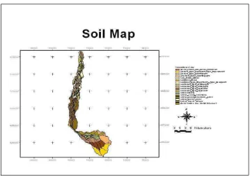
4.1.3 Soil……….
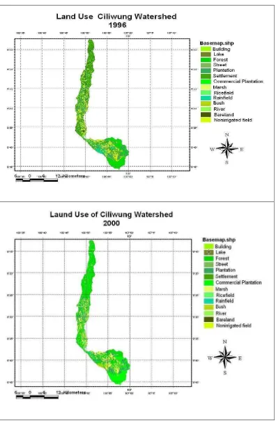
4.1.4 Landuse Change………
4.1.5 Water Level………
4.1.6 Model Calibration………..
4.1.7 Model Structure……….
4.2 Disscusion……….
4.2.1 Physical and Environtment Condition………...
4.2.2 Climate………..
4.2.3 Soil……….
4.2.4 Landuse Change……….
4.2.5 Water Level………
4.2.6 Model Calibration and Validation……….
4.2.7 Model Structure……….
4.3 Model Simulation using Scenario……… 39
41
42
45
47
49
52
52
53
53
54
55
55
56
56
V. CONCLUSION AND RECOMENDATION
5.1 Conclusion………...
5.2 Recommendation……….
61
62
MODELING OF FLOOD FOR LAND USE MANAGEMENT
(Case Study of Ciliwung Watershed)
I PUTU SANTIKAYASA
GRADUATE SCHOOL
MODELING OF FLOOD FOR LAND USE MANAGEMENT
(Case Study of Ciliwung Watershed)
I PUTU SANTIKAYASA
A Thesis submitted for the degree of Master of Science of Bogor Agricultural University
MASTER OF SCIENCE IN INFORMATION TECHNOLOGY
FOR NATURAL RESOURCES MANAGEMENT
GRADUATE SCHOOL
STATEMENT
I, I Putu Santikayasa, here by stated that this thesis entitled
Modeling of Flood for Land Use Management
(Case Study of Ciliwung Watershed)
are result of my own work during the period February 2005 until April 2006 and
that it has not been published before. The content of the thesis has been examined
by the advising committee and the external examiner.
Bogor, August 2006
ACKNOWLEDGMENT
All the praises and thanks be to Hyang Widhi, The Lord of Heaven. The
title of the research, which was held in January to September 2005 is “Modeling
of Flood for Land Use Management (Case Study of Ciliwung Watershed)”.
I would like to thank to Dr. Ir Handoko, M.Sc as my supervisor, for the
guidance and encouragement during research and also for providing scholarship
for my study, Dr. Ir. Hartrisari, H. as my co-supervisor for the guidance and
encouragement during research and Dr. Yuli Suharnoto as the examiner of this
thesis for the positive ideas and inputs.
I would like to thank to all MIT secretariat that support our administration,
technical and facility. I would also thank to all MIT lecturer who taught me with
very important knowledge during my study. Thank you to Idung Risdiyanto,
M.Sc, for programming guidance and also thank you to Supri for data support.
High appreciation goes to Bogor Agriculture University, SEAMEO
BIOTROP, Bioresources Management Center (BrMC) for the facilities
exspecially computer of this study.
I would like also thank to all my colleagues in Department of Geophysics
and Meteorology, IPB. To all my friends in Asrama Bali, thank for your support.
CURRICULUM VITAE
I Putu Santikayasa was born in Pohsanten, Jembrana - Bali at February 24, 1979.
He received his undergraduate from Bogor Agricultural University in 2002 in the
field of Agrometeorology. Since 2005 until now, He works as lecturer in
Department of Geophysics and Meteorology, Faculty of Mathematics and Natural
Sciences, Bogor Agricultural University.
In the year 2003, he a scholarship from SEAMEO BIOTROP to continue his
study for master degree in MIT IPB. He receive his Master of Science in
Information Technology for Natural Resources Management from Bogor
Agriculture University in 2006 respectively. His thesis was on title “Modeling of
ABSTRACT
I PUTU SANTIKAYASA(2006). Modeling of Flood for Land Use Management (Case Study of Ciliwung Watershed). Under the supervision of Handoko and Hartrisari.
Floods are one of the major disasters affecting many countries in the world year after year. It is an inevitable natural phenomenon occurring from time to time in all rivers and natural drainage systems. It causes damage to lives, natural resources and environment as well as the loss of economy and health. Floods represent complex problems because of its variety. Therefore, this variety cannot be studied or controlled only by one or two specific methods.
The objectives of this research are to understand the process of flood events and its interaction with hydrometeorological components, to develop flood model for watershed management and to determine the effect of land use change to watershed discharge which indicates flood event.
The research consists of four processes those are 1) Data Preparation, 2) Model Development, 3) Model Simulation and 4) Model Calibration and Validation. Data preparation was conducted for two kinds of data namely spatial data and tabular data. Model developed as numerical model of the hydrology of a river basin system. This model includes the response of watershed to precipitation, the actions of the river network as water flows through the river, the effect of land use changes, and the effect of engineering structures to the watershed. Model simulated by change land use as an input. Model calibrated by using water level data of field measurement in year 1996 and model validated by using water level data of field measurement in year 2000.
Research Title : Modeling of Flood for Land Use Management (Case Study of Ciliwung Watershed)
Student Name : I Putu Santikayasa
Student ID : G 051024021
Study Program : Master of Science in Information Technology for Natural Resources Management
Approved by,
Advisory Board:
Dr. Ir. Handoko, M.Sc Dr. Ir. Hartrisari H.
Supervisor Co-Supervisor
Endorsed by,
Program Coordinator Dean of the Graduate School
TABLE OF CONTENTS
Page
STATEMENT ……….
ACKNOWLEDGMENT ……….
CURRICULUM VITAE ……….
ABSTRACT ………
TABLE OF CONTENT ………..
LIST OF TABLE ……….
LIST OF FIGURE ……… i ii iii iv v vi vii I. INTRODUCTION
1.1 Background ………
1.2 Objective……….
1.3 Hypothesis………...
1.4 Thesis Structure………... 1
4
4
4
II. LITERATURE REVIEW
2.1 Watershed………..
2.1.1 Watershed Definition………..
2.1.2 Watershed as a System………..
2.1.3 Watershed Modeling……….
2.1.4 Watershed and Drainage Basin……….
2.1.5 Basin Characteristics Affecting Runoff……….
2.2 Process-Based Hydrology Modeling……….
2.2.1 Hydrology Cycle………...
2.2.3 Hydrometeorology Component………
2.2.4 Classification of Hydrology Modeling………..
2.3 Flood………..
2.3.1 Flood Definition………
2.3.2 Flood Routing………
2.3.3 Flood Modeling……….
2.3.4 Step in Hydrology Modeling Development………..
2.4 Land Use Effect Runoff……….
2.5 The Infuenced of Land Use Management on Flood Risk………….. 13 16 17 17 18 20 21 22 23
III. RESEARCH METHODOLOGY
3.1 Time and Location of research………..
3.2 Data Collection……….
3.3 Required Tools……….
3.3.1 Software……….
3.3.2 Hardware………
3.4 Method……….
3.4.1 Data Preparation………
3.4.2 Model Development………..
3.4.2.1 Model Description……….
3.4.2.2 Model Construction………...
3.4.3 Model Calibration and Validation………. 25 26 26 26 26 27 27 27 27 29 37
IV. RESULT AND DISCCUSION
4.1 Result……….
4.1.1 Physical and Environtment Condition………... 38
4.1.2 Climate………..
4.1.3 Soil……….
4.1.4 Landuse Change………
4.1.5 Water Level………
4.1.6 Model Calibration………..
4.1.7 Model Structure……….
4.2 Disscusion……….
4.2.1 Physical and Environtment Condition………...
4.2.2 Climate………..
4.2.3 Soil……….
4.2.4 Landuse Change……….
4.2.5 Water Level………
4.2.6 Model Calibration and Validation……….
4.2.7 Model Structure……….
4.3 Model Simulation using Scenario……… 39
41
42
45
47
49
52
52
53
53
54
55
55
56
56
V. CONCLUSION AND RECOMENDATION
5.1 Conclusion………...
5.2 Recommendation……….
61
62
LIST OF FIGURES
Figure 1. Physical Characteristics Of Watershed...7
Figure 2. Conceptual of Hydrologic Cycle Diagram ...11
Figure 3. Relationship of each Hydrologic Component ...16
Figure 4. Flood in Jakarta ...19
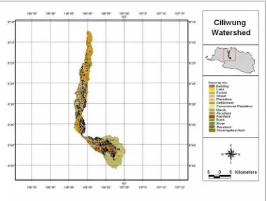
Figure 5. Map of Study Area ...25
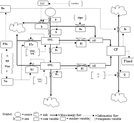
Figure 6. Forester Diagram of Flood Modeling ...29
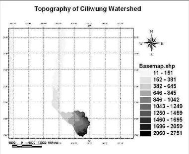
Figure 7. Topography map of Ciliwung Watershed ...39
Figure 8. Daily (left) and Monthly (right) Precipitation of Ciliwung Watershed..40
Figure 9. Monthly average temperature (left) and relative humidity (right) ...41
Figure 10. Soil Map of Ciliwung watershed ...41
Figure 11. Land Use Map of Ciliwung Watershed in year 1996 and 2000 ...43
Figure 12. Land Use Change of Ciliwung Watershed in year 1996 and 2000 ...44
Figure 13. Water Level in Manggarai and Area Precipitation in Ciliwung Watershed... 45
Figure14. Measured water level in 1996 and 2000...46
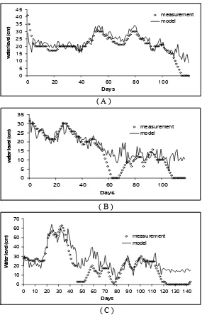
Figure 15 The simulated and observed water level in location, year : (A) Katulampa, 1996 ; (B Depok, 1996; (C) Manggarai, 1996... 47
Figure 16 The simulated water level in location: (A) Katulampa (B) Depok (C) Manggarai ... 48
Figure 17. Main Window of Flood Model...50
Figure 18. Land Use Map Of Ciliwung Watershed For Each Scenario; (A) Urbanization, (B) Deforestation, (C) Afforestation, (D) Present... 58
Figure 19. Simulated Hydrograph For Each Scenario in Manggarai...59
LIST OF TABLES
Table 1. Percentages of Interception by Various Crops and Grass... 14
Table 2. Effect Of Some Landuse Treatment And Treatment Measure On The
Direct Runoff ... 23
Table 3. List of data Required in developing Flood Model ... 26
Table 4. Soil Type of Ciliwung Watershed... 42
Table 5. Input Data of Flood Model... 49
Table 6. Output of Flood Model ... 49
Table 7. Toolbar of the Interface... 51
Table 8. Menu on the Interface ... 51
I.
INTRODUCTION
1.1 Background
Floods are one of the major disasters affecting many countries in the world
year after year. It is an inevitable natural phenomenon occurring from time to
time in all rivers and natural drainage systems. It causes damage to lives, natural
resources and environment as well as the loss of economy and health.
According to Islam (2002), in recent decades, floods losses have increased
worldwide. This can be linked to socio-economic, hydrological and climatic
factors. An increase of flood risk is also foreseen for the future. Several landuse
changes, such as deforestation and urbanization, reduce the available water
storage capacity and increase the flood hazard.
Flood is becoming an increasing major contributor to personal and to
property damage worldwide and in many places strikes without warning.
Increasing population pressure and economic activities has led to the development
of extensive infrastructures near the rivers. These economic activities and land
use changed increase the risk of future inundations.
Floods represent complex problems because of its variety. Therefore, this
variety cannot be studied or controlled only by one or two specific methods. In
this case, flood has been viewed as a system that integrates any discipline by
including social discipline.
In Indonesia, climate change especially of extreme rainfall, caused by La
have greatly increased and there is a need for effective modeling and
understanding of the problem to help mitigate the worst effects of flood disasters
and the need for developing a system to understand the threatened areas. The
understanding of process will help in flood hazard assessment and in giving
insights to various ways of dealing with the hazard and disaster problems.
Ciliwung River is one of the biggest rivers which passes Jakarta and
eventually causes flood in Jakarta. In the first year of 1996, Ciliwung River
causes flood in Jakarta and damage. In year 2002 the flood event was bigger than
previously and causing damage about 40 % of Jakarta area (BPS Jakarta).
The land use of Ciliwung watershed has been changed in the last 25 years.
This change increases runoff of about 54 %. This runoff change has high
correlation with the land use change in the Ciliwung watershed (Fakhrudin,
2003).
Land use change affects hydrological characteristics such as infiltration,
surface storage, and evapotranspiration. The decrease of infiltration will increase
runoff. This condition is potential to cause flood in the wet season while causes
drought in the dry seasons. Surface storage has a correlation with time lag of
runoff. The decrease of surface storage will increase runoff flow which means the
water has no time to infiltrate but directly flows to the river and causes flood in
low places.
Flood is a dynamic system because flood process is time dependent.
Dynamic system is described by time-differential equations; therefore, the
(the initial conditions) and the present input. Thus, a dynamic system may
continue to have a time-varying response after the inputs are held constant.
As a dynamic process flood event can be forecasted. One method to
forecast flood events is by considering flood process as a system. As a system,
flood process has component such as input, process, output, feedback process,
environment, and boundary. The important factor from system is its behavior.
The behavior will provide the explanation of flood event and bring it to the
solution. By changing the value of variables during simulation it also gives the
effect degree of each component. This is very important to make decision related
to the action in the field.
Geographic information system (GIS) provides a broad range of tools for
determining area affected by floods and for forecasting areas that are likely to be
flooded due to high water level in a river. Prahasta (2001) also mentioned that
GIS is the nucleus of the environmental information system. Most of the
information needed to operate an urban is geo-referenced, i.e. it is referenced to
specific geographic location. Information about zoning, properties, roads, rivers,
administration boundary are connected to geographic locations.
Based on the explanation above, this research will study hydrology
response to land use change and modeling flood event by using system dynamic
approach. The benefit of this model is that the model can explain flood process
and its behavior and can be used to evaluate watershed system. This model will be
used as a tool to evaluate the effect of land use change to the water level in the
1.2 Objectives
The objectives of this research are :
• To understand the process of flood events and its interaction with
hydrometeorological components.
• To develop flood model for watershed management
• To determine the effect of land use change to watershed discharge which
indicates flood event.
1.3 Hypothesis
• Land use change influence discharge in the outlet.
1.4 Thesis Structure
The thesis consists of six consecutive chapters. The contents of each
chapter are described below:
• Chapter I introduces the research by focusing on the background such as
introduction, objectives, hypothesis, and thesis organization.
• Chapter II provides comprehensive summary of related work ranging
from watershed, process-based hydrological modeling, flood, and
landuse management.
• Chapter III introduces the study area, materials and methods.
• Chapter IV focuses on the results and discussion. This chapter includes
of study area characteristics and model structure, model calibration, and
model profile.
II.
LITERATURE REVIEW
2.1 Watershed
2.1.1 Watershed definition
The term watershed describes an area of land that drains downslope to the
lowest point. The water moves through a network of drainage pathways, both
underground and on the surface. Generally, these pathways converge into streams
and rivers, which become progressively larger as the water moves on downstream,
eventually reaching an estuary and the ocean. Other terms used interchangeably
with watershed include drainage basin or catchments basin.
Watersheds can be large or small. Every stream, tributary, or river has an
associated watershed, and small watersheds join to become larger watersheds. It
is relatively easy to delineate watersheds using a topographic map that shows
stream channels. Watershed boundaries follow major ridgelines around channels
and meet at the bottom, where water flows out of the watershed, a point
commonly referred to as a stream or river.
The connectivity of the stream system is the primary reason for doing
acquatic assessments at the watershed level. Connectivity refers to the physical
connection between tributaries and the river, between surface water and
groundwater, and between wetlands and water. Because water moves
downstream, any activity that affects the water quality, quantity, or rate of
everyone living or working within a watershed needs to cooperate to ensure good
watershed conditions.
2.1.2 Watershed as a System
Watershed as a system consider the form and appearance of a typical
watershed, illustrated in the Figure 1. Included in this Figure are some of the
physical characteristics of a typical watershed.
Figure 1. Physical Characteristics Of Watershed Source : http://www.sbg.ac.at/geo/idrisi/gis_environmental_modeling/
sf_papers/collins_fred/collins.html
From the Figure above, the amount of water in a river depends on the
inputs and the outputs. The inputs are water flowing over the surface water
seeping in through the bed of the stream from the soil and/or groundwater
(although in arid regions, this second inflow is actually an outflow; the stream lies
above the water Table and loses water to the soil and ground water). The flow of
and most streams are maintained by this ground water and soil water contribution.
Water leaves the river by flowing down the channel; this rate is controlled by
stream parameters like the gradient of the stream, the roughness of the stream bed,
and the shape of the channel. The shape of the channel is important since it
determines what portion of the flowing water is in contact with the stream bed and
can thus be slowed by friction associated with the rough surface of the stream bed.
2.1.3 Watershed Modeling
Watershed modeling encompasses processes that make up the land portion
of the hydrologic cycle. Such models track the flow of water from rainfall inputs
to infiltration, seepage to groundwater, overland flow, channel flow, subsurface
stormflow, and evapotranspiration. Models that simulate a single
precipitation/runoff event are called event based models, while models that can
simulate processes occurring between Precipitation events are called continuous
simulation models. If watershed models only have one parameter value for a
given watershed or sub watershed, the model is referred to as a lumped-parameter
model. If the model allows for multiple location values for a given parameter
within a watershed or sub watershed, the model is referred to as a distributed
model.
Watershed models can be further categorized as either conceptual models
or physics-based models. Conceptual models make use of idealizations of
processes in the simulation of watershed phenomena. For example, a conceptual
model may simulate the watershed as a collection of reservoirs connected in series
watershed processes. In such model, there may be a reservoir for groundwater, a
reservoir for infiltrated water, a reservoir for water in channels, and a reservoir for
overland flow water. Water is moved from one reservoir to another to simulate
the precipitation-runoff process. The rules for transferring water from one
reservoir to another are based on a parameterization of the particular process (e.g.
infiltration moving precipitation to sub-surface storage or groundwater). Such
models are useful for viewing at total watershed response (runoff at the outlet of
the watershed). These models rely on observed data for calibration of the
parameters that govern the movement of water between the different components.
Parameters are changed until the modeled runoff at the outlet of the watershed
matches the observed runoff. In some conceptual models there are possibilities of
matching modeled to observed data in the interior of the watershed as well.
An alternative to conceptual models are physics-based watershed models.
In general, these are the most complex of watershed models as they utilize
conservation equations (conservation of mass, momentum, or energy) to simulate
watershed processes. As an example, physics based models may use versions of
the shallow water equations (conservation of mass and momentum) like the
diffusion wave to simulate channel flow or overland flow. Movement of water
through each part of the land portion of the hydrologic cycle is governed by a
conservation equation in one, two or three dimensions. Initial and boundary
conditions are required to solve the equations and provide linkages between the
different processes. The parameters of physics-based models are either
based models can be estimated directly from field data and land features, negating
the requirement of historical concurrent precipitationl-runoff data for their
calibration.
2.1.4 Watershed and Drainage Basin
Streams and rivers convey both surface runoff and ground water flow
away from high water areas, preventing surface flooding and rising groundwater
problem. A watershed area supplies surface runoff to a river stream, whereas a
drainage basin for a given stream is the fact of land drained of both surface runoff
and groundwater discharge.
Surface runoff from a watershed flows downhill until reaching a tributary
or stream. The lines separating the land surface into watershed are called divides.
These normally follows ridges and mounds and can be delineated using contour
maps, fields surveys, or stereograph pairs of areal photographs to identify gradient
directions.
2.1.5 Basin Characteristics Affecting Runoff
The nature of stream flow in a region is a function of hydrologic input to
the region and the physical, vegetative, and climatic characteristic. As indicated
by the hydrologic equation, all the water that occurs in an area as a result of
precipitation does not appear as stream flow. Fractions of the gross precipitation
are diverted into paths that do not terminate in the regional surface transport
system. Precipitation striking the ground can go into storage on the surface or in
that influences runoff are: 1) geologic consideration, 2) stream pattern, and 3)
geomorphology of drainage basin.
2.2 Process-Based Hydrology Modeling
2.2.1 Hydrology Cycle
The hydrology cycle is a continuous process by which water is transported
from the oceans to the atmosphere then to the land and back to the sea. Many
sub-cycles exist inside. The driving force for the global water transport system is
provided by the sun, which furnishes the energy required by evaporation.
Because the total quantity of water available to the earth is finite and
indestructible, the global hydrologic system may be looked upon as closed system.
Open hydrologic sub systems are abundant, however and these are usually the
type analyzed. For any system a water budget can be developed to account for the
hydrologic component. The process of hydrologic cycle describe as Figure below
:
Figure 2. Conceptual of Hydrologic Cycle Diagram
2.2.2 Physically Based Hydrological Models
The physically based models are based on our understanding of the
physics of the hydrological processes which control the catchments response and
use physically based equations to describe these processes. A discretization of
spatial and temporal coordinates is made and the solution is obtain hydrological
applications has broadened dramatically over the past four decades. Although the
problems of flood protection and water resources management continue to be of
importance and relevance for the security of communities and for human, social
and economic development, many applied problems relating to the wider role of
hydrology have come into focus.
Physically based distributed models of the hydrological cycle can in
principle be applied to almost any kind of hydrological problem. These models
are based on our understanding of the physics of the hydrological processes which
control catchments response and use physically based equations to describe these
processes. Some typical examples of field applications include study of effect of
catchments changes, prediction of behavior of ungauged catchments, of spatial
variability in catchments inputs and outputs, movement of pollutants and
sediment.
Hydrological modeling is a powerful technique of hydrologic system
investigation for both the research hydrologists and the practicing water resources
engineers involved in the planning and development of integrated approach for
management of water resources. Physically based distributed models do not
consider the transfer of water in a catchments to take place in a few defined
models can simulate the complete runoff regime, providing multiple outputs (e.g.
river discharge, phreatic surface level and evaporation loss) while black box
models can offer only one output. In these models transfer of mass, momentum
and energy are calculated directly from the governing partial differential equations
which are solved using numerical methods. As the input data and computational
requirements are enormous, the use of these models for real-time forecasting has
not reached the ‘production stage’ so far.
Physically-based distributed models can in principle be applied to almost
any kind of hydrological problem. Some examples of typical fields of application
are catchments changes, ungauged catchments and spatial variability.
2.2.3 Hydrometeorology Component
Precipitation
Precipitation is the primary input vector of the hydrologic cycle and the
most important input into a simulation model of the land phase of hydrological
model. Precipitation is derived from atmospheric water, its form and quantity thus
being influenced by the action of the climatic factor such as wind, temperature
and atmospheric pressure.
Interception
Interception is defined as the process whereby precipitation is retained on
the leaves, branches, and steams of vegetation and on the litter covering the
Some observed percentages of interception by various crops and grasses
shown as Table 1.
Table 1. Percentages of Interception by Various Crops and Grass
Vegetation Vegetation Type Intercepted (%)
Crops Alfalfa
Corn Soybeans Oats 36 16 15 7 Grasses Little Bluestem
Big Bluestem Tall panic grass Bindweed Buffalo grass Blue grass Mixed species Natural grasses 50-60 57 57 17 31 17 26 14-19
source: O. R. Clarck (1937)
Evaporation and Transpiration
Evaporation is the transfer of water mass from the liquid to the vapor state.
Transpiration is a plant metabolism process where water is received from the soil
and released as vapor to the atmosphere. Evapotranspiration take place from
water, snow, land, and vegetation surface. The volume of water which leaves the
land phase of the hydrologic cycle by actual evaporation and transpiration in the
most cases exceeds that which flows to the oceans by runoff.
Radiation
The processes by which the sun’s energy reaches the surface of the earth
are complex. Radiation is one form of energy transfer. From a hydrologic
viewpoint, the important forms of solar energy reaching the surface of the earth
radiation, and long-wave atmospheric radiation, all in downward direction; and
reflected components of short-wave radiation and the long-wave terrestrial
radiation emitted by the surface of the earth.
Wind speed and direction
Both wind speed and direction are important for calculating another
atmosphere processes. Wind speed is important for calculating evaporation,
snow melt, or rain gauge loses. Wind direction can be used to estimate flow of
water vapor.
Cloud cover
Cloud cover affects the transfer of energy to the land surface by
intercepting part of the direct sort-wave radiation. Cloud cover observations are
important in situations where no observations exist on incoming radiation. In
such cases, estimated values of clear sky radiation are used with adjustments for
affect of cloud cover.
Stream flow
Stream flow records provide a measure of the response of a catchments to
the time variable input and internal hydrologic processes. These records are used
in simulation techniques during model calibration to assess the dominant
processes contributing to the response of base flow and overland flow. Figure
Figure 3. Relationship of each Hydrologic Component Source : http://www.sbg.ac.at/geo/idrisi/gis_environmental_modeling/
sf_papers/collins_fred/collins.html
2.2.4 Classification of Hydrology Modeling
Watershed models are developed for different purposes. Nevertheless
many of those model share structural similarities, because their underlying
assumptions are the same, and some of the models are distinctly different. The
watershed models can be classified according to different criteria that encompass
process description, scale, and technique of solutions.
The watershed model can be classified based on the time scale of models.
One of the time intervals is used for input and internal computations. The second
is the time-interval used for the output and calibration of the model. Based on
these description, the models can be classified as 1) continuous-time or event
The watershed can also classified depend on the space of watershed.
These criteria is use to classify into small watershed, medium size watershed, and
large watershed. For consideration of runoff generation on these watersheds, two
phases can be considered: 1) land phase and 2) channel phase. Large watersheds
have well developed channel network and channel phase, and thus, channel
storage is dominant. The other hand, small watershed have dominant land phase
and overland flow, have relatively less conspicuous channel phase, and are highly
sensitive to high- intensity, short-duration rainfalls.
Watershed can be classified base on land use. Watershed can be classified
into agriculture, urban, forest and range land, desert, mountain, coastal, wetlands
and mixed area. In many case, large or even medium size of watersheds have
mixed land use. These watersheds behave hierologically differently, indeed so
differently that they have given rise to different branches of hydrology.
And frequently watershed model classified on the basis of their intended
use. Model are classify into: 1) planning models, 2) management models, and 3)
prediction models. A comprehensive watershed model can be employed to
accomplish a considerable array of analytical tasks for planning and management
of water resources (Viesman, 1989).
2.3 Flood
2.3.1 Flood Definition
Flood is defined as any relatively high flows that overtop the natural or
artificial banks in any reach of a stream. When the banks are overtopped, water
Flood may be measurable as to height, area inundated, peak discharge, and
volume of flow. The height of a flood is of interest to those planning of build
structure along or across streams; the area inundated is of interest to those
planning to occupying in any manner the floodplains adjacent to a streams; the
peak discharge is of interest to those designing spillways, bridges, culverts, and
flood channel; and the volume of flow is interest to those designing storage works
for irrigation, water supply, and flood control.
Floodplains are areas with ecologically important wetlands, and mainly
exhibit competitive advantages for human urban. Resolving the potential conflict
between ecological value and human use is consequently a major issue in
determining the most appropriate flood hazard management strategy.
2.3.2 Flood Routing
Flood routing defined as the procedure whereby the time and magnitude of
a flood wave at a point on a stream is determined from the known or assumed data
at one or more points upstream.
The movement of a flood wave down a channel or through a reservoir and
the associated change in timing or attenuation of the wave constitute an important
topic in floodplain hydrology. It is essential to understand the theoretical and
practical aspects of flood routing to predict the temporal and spatial variations of a
flood wave through a river reach or reservoir. Flood routing methods can also be
used to predict the outflow hydrograph from watershed subjected to a known
Routing technique may be classified into two major categories: simple
hydrologic routing and more complex hydraulic routing. Hydrologic routing
involves the balancing of inflow, outflow and the volume of storage through use
of the continuity equation. Hydrologic routing can be used in flood prediction,
flood control measures, reservoir design and operation, watershed simulation, and
urban design. Whereas hydraulic routing method is based on the solution of the
continuity equation and the momentum equation for unsteady flow in open
channel. Hydraulic routing method is used in case: upstream movement of tides
and storm surge, backwater effect from downstream reservoir and tributary
inflows, flood waves in channels of very flat slope, and abrupt wave caused by
sudden releases from reservoir or dam failure.
2.3.3 Flood Modeling
The first step in risk management for floods is the flood hazard mapping.
For planning and evacuation procedures, the demand for flood information and
digitals maps of predicted extent and risk of flooding has been increased. To
produce these maps Geographical Information System (GIS), Remote Sensing
(RS) and flood modeling is very useful.
Simulation and modeling of flood are a rapidly developing field in
hydrology. The flood simulation and model results are a good way of providing
relevant information on how the flood is going to behave at the location where
people live and how the flood will affect them.
There are many types of flood models, 1-dimensional (1D) floods models
such as manning equation, HEC-2, and dynamic one-dimensional model such as
SOBEK, MIKE-11 have been used to estimate the possible flood using time series
of river discharge. 1-D model has some limitation on include all details in
modeling and it is very difficult to simulate local conditions on a small scale
accurately (Singh, 1995)
Two dimensional (2D) modeling based on the raster grids for terrain
description, surface roughness coefficients and hydrological data (water level,
discharge and cross section) provide information to generate flood hazard maps.
Over the past ten years significant advances have been made in integrating
1D and 2D models resulting in hydrodynamic model of floodplains and integrated
1D (channel flow) and 2D ( overland flow). The idea of integrating 1D
hydrodynamic modeling technologies, Digital Elevation Model (DEM) and GIS
them in the GIS as maps. Benefit of the integration of GIS, RS, 2D flood
modeling is to provide information for users such as land use planning, evacuation
planning and environmental impact assessment.
2.3.4 Step in Hydrology Modeling Development
A simulation model is a set of equations and algorithm that describe the
real system and imitate the behavior of the system. A fundamental first step in
organizing a simulation model involves a detailed analysis of all existing and
proposed components of the system and the collections of relevant data. This step
is called the system identification or inventory phase. Included items of interest
are site locations reservoir characteristics, precipitation and stream flow histories,
water and power demands, and so forth.
The second phase is model conceptualization, which often provides
feedback to the first phase by defining actual data requirements for the planner
and identifying system components that are important to the behavior of the
system. This step involves 1) selecting a technique that are to be used to represent
the system elements, 2) formulating the comprehensive mathematics of the
techniques, and 3) translating the proposed formulation into a working computer
program that interconnects all the subsystems and algorithm.
Following the system identification and conceptualization phases are
several steps of the implementation phase. These include 1) validating the model,
2) modifying the algorithms as necessary to improve the accuracy of the model,
2.4 Landuse Effects on Runoff
Watershed is the hydrology system which include the component of input,
processes, and output. The primary input is precipitation and by the process in the
watershed, excess water from precipitation will become channel outflow in the
outlet. If process in the watershed “normal”, the fluctuation of channel flow will
not be significant.
Hydrology process in the watershed influence by geomorphology,
geology, topography, climate, soil, and landuse factor. Those factor relate each
other and land use is the factor which change faster compare with the other factor.
Landuse changed caused by the increasing of population and socio-economic.
Runoff processes if amount of precipitation larger than rate of infiltration,
interception and soil water storage. Increasing rate of infiltration will decreasing
runoff. The rate of infiltration influenced by such factor as the type and extent of
vegetation cover, the condition of surface layer, temperature, rainfall intensity,
physical properties of the soil, and water quality. The water at which water is
transmitted through the surface layer is highly dependent on the condition of the
surface. The volume of storage available below the ground is also a factor
affecting infiltration rates.
Modification of the land surface have varying effects on the runoff
characteristics. For example if a heavily forested area with its thick layer of
mulch is converted to cropland or pasture, the soil is disturbed and the overlying
absorptive cover is changed. The result is increased runoff volume and a change
is timing of flows. When lowlands or marshes are surface drained, the flooding
infiltration capacities of soils and landuse changes that modify the nature of
vegetation can have significant impact on the timing and volume of flows.
The principle effects of landuse change have been classified by Leopold
(1968) as follows: 1) changes in peak flow characteristics, 2) changes of total
runoff, 3) changes of water quality, and 4) changes in hydrologic amenities (the
appearance or impression a watercourse)
Land use change can increase or decrease the volume of runoff and the
maximal rate and timing of flow from a given area. The most influential factors
affecting flow volume are the infiltration and surface storage. If the landuse
change decrease flow volume also decrease the peak rate of flow and vice versa.
Some effect of landuse treatment on the direct runoff are shown in the Table
below:
Table 2. Effect Of Some Landuse Treatment And Treatment Measure On The Direct Runoff
Reduction in direct runoff volume Effect
Measure
Increasing infiltration rate
Increasing Surface Storage
Landuse change that increases plant or root density √ Increasing mulch of litter √
Contouring √
Contouring furrowing √
Level terracing √
Graded terracing √
Source: Bras (1990)
2.5 The Influenced of Land Use Management on Flood Risk
Catchments landscapes are complex mosaics of land use and land
functioning and flood responses, but the way in which these diverse influences
combine to generate the flood hydrograph and flood frequency curve at increasing
catchments scales is not well understood. Typical influences which can impact
local scale flood responses include soil compaction in fields, resulting in reduced
porosity and infiltration, the acceleration of sub-surface runoff through field
drains, enhanced flow connectivity pathways through ploughing ditches etc.
While various measures might be taken to counteract these effects, their potential
impact on large scale flood responses needs to be investigated through a
combination of field experiments and modeling
Bad land use management practices are thought to be the cause of
increased flooding. This result when land use decisions not taking into account
the effect of development on the water resources of the basin are implemented.
Since there are economic consequences involved in flooding issues it
becomes important to assess the flood risks in a basin and where possible to
minimize those risks in order to reduce costs. This is a concern for individuals,
private enterprises and governments who bears the cost of floods when they occur.
It is also true that damages to flooding tend to be inequitable affecting
those who likely have no control of the situation and even without any
compensation. When bad land use practices occur upstream they affect
homeowners, farmers and communities downstream with increased flooding
potential, more sedimentation, polluted water and reduced water availability. It is
therefore important to understand the role of land use changes on flooding risks at
local scale such that political and technical measures can be taken to reduce the
III.
RESEARCH METHODOLOGY
3.1 Time and Location of Research
This research was conducted in Bogor from September 2004 until October
2005. Location of the research is Ciliwung watershed. That is located between
06o 05’ S – 06o 55’ S and 106o 40’ E – 107o 00’ S. Location of the study is shown
[image:47.612.133.514.298.585.2]in Figure 5.
3.2 Data Collection
Three types of data will be needed in this research, i.e. Ciliwung watershed
spatial data, water level data, and statistical data of climate. Those data are listed
[image:48.612.134.508.202.403.2]as follows:
Table 3. List of data Required in developing Flood Model
No Data Format
1. The spatial data of Ciliwung watershed in ESRI format.
• Landuse/Landcover • Soil Type
• Contour • River
Digital (*.shp)
2. Water level data of watergate station Hardcopy/printed
3. Climate data Digital (*.csv)
3.3 Required Tools 3.3.1 Software
In this research, some supporting tools of software and hardware were
used :
• ESRI ArcView version 3.x plus extension
• Microsoft Visual Basic 6
• ESRI Map Object 2.x • Microsoft Access
• Microsoft Visio • Microsoft Excel
3.3.2 Hardware
3.4 Method
The research consists of four processes those are 1) Data Preparation, 2)
Model Development, 3) Model Simulation and 4) Model Calibration and
Validation.
3.4.1 Data Preparation
Data preparation was conducted for two kinds of data namely spatial data
and tabular data. Preparation of spatial data converts vector data format to raster
data format with size 30 m x 30 m. Process of converting data from vector to
raster uses spatial analysis and 3D analysis of ArcView extension. Raster format is
needed by each process of hydrology calculation because each calculation should
be conducted in each cell.
Preparation of tabular format was made to the attribute of shape file. The
process divides each theme into one Table. This format is called “one cell many
table”. Converting process was done by using Microsoft Excel and Microsoft
Access.
3.4.2 Model Development
3.4.2.1Model Description
This model is a numerical model of the hydrology of a river basin system.
This model includes the response of watershed to precipitation, the actions of the
river network as water flows through the river, the effect of land use changes, and
the effect of engineering structures to the watershed. The computation center for
the program is in two main modules, the watershed module and the river system
submodel will become input for the river system submodel and also computation
result from the river system submodel become input for watershed submodel.
These are interfaced by numerous utility programs and several databases,
providing the user with a variety optional configurations and applications in
setting up the programs.
A. Watershed submodel
Watershed module simulates precipitations, interceptions, and the state of
soil system as it affects runoff, the effect of land use changes, and the translation
of runoff in several components to the stream system. Evapotranspiration and
long-term soil moisture routing was accounted for making it possible to simulate
continuously throughout several year period in low as well as high flow
conditions.
B. River submodel
River module simulates the routing of streamflow through a river. Several
variations in specifying channel routing methodology are available, including the
provision to account for backwater effects from independent downstream sources.
This module also contains the algorithms for simulating reservoir operations, and
3.4.2.2Model Construction
The model constructed by following the processes of water cycle. The
boundary of the model is the watershed boundary. The source is precipitation (P)
over the watershed. The mass flow is water, and the sinks are atmosphere for
evapotranspiration and the next channel for channel outflow.
[image:51.612.111.537.255.648.2]The processes in the model shown as forester diagram in Figure 6.
Figure 6. Forester Diagram of Flood Modeling P Ic SWC1 Ro If1 ETa SWC2 Pc1
Tr2 If2
Af1 Af2 CF Is Pc2 slope Landuse ETm Wind RH Q T Tm Ea Em LAI Flood Q SWC1 WP1 SWC2 WP2 Cr A
Some of the precipitation (P) are intercepted by trees, grass, other
vegetation, and structural objects. Precipitation (P) data are generated from point
precipitation depth in the precipitation gauge as a point data. Spatial precipitation
is generated by interpolating point precipitation data from each precipitation
gauge by using isohyets method.
Area precipitation is calculated by using the following equation:
i
iP
A
P=Σ ……… ………. ……….(1)
Where Ai is the area of each isohyet and Pi is the precipitation of the isohyets.
Interception (Ic) is influenced by vegetation parameter that is Leaf Area
Index (LAI) and Precipitation. The value of Ic is determined by Zinke (1967) as
the following equation:
LAI Ic = 3 2 . 1 3
0<LAI < …………..………...(2)
2 . 1 =
Ic LAI ≥3
P
Ic= P<Ic
Precipitation occurring over the watershed falls on two types of surfaces
which are a portion of the upper zone. These are, 1) a permeable portion of soil
mantle, and 2) a portion of soil mantle covered by stream, lake surfaces, marshes,
rock, pavement, or other impervious material which is or becomes linked to the
stream as soil moisture increases. Both of them produce runoff (Ro). Ro of the
first area will be produced when precipitation is heavy, while the second area
produces Ro from the portion of the watershed which is actively impervious. Ro
is influenced by slope, precipitation netto, extractable water (EW), field capacity
) (
% %
75 slope Stft EW
Ro= × × − Stft > EW; ……….………(3)
Stft Slope
Ro=75%×% × θ(1) > Fc(1)
The remaining P will be infiltrated before filling the ground. The
infiltration rate (mm d-1) equals to precipitation minus interception and runoff.
Infiltration (Is) is calculated by the difference between precipitation and canopy
interception(Penning de Vries F.W.T. et al. 1989; Handoko, 1994)
Ro Stft
Is= − ………(4)
Not all water that reaches the surface infiltrates the soil surface, especially
during heavy rain. Runoff from a field can be 0-20 % of precipitation, and even
more on unfavorable surfaces (Penning de Vries F.W.T. et al. 1989). Runoff
occurs when the rate of water supply at the soil surface exceeds the maximum
infiltration rate.
Infiltration process change surface soil water content or Soil Water
Content Layer 1 (SWC1). SWC1 represents the balance input from precipitation
and losses of water including interflow (If1) and surface percolation (Pc1).
The water balance equations which represent soil water content for upper
and lower layer on day t are:
t t
t t t
t(1)=θ−1(1)+Is −Pc (1)−Tr(1)−Ea
θ ) 2 ( ) 2 ( ) 1 ( ) 2 ( ) 2
( =θt−1 +Pct −Pct −Trt
Interflow (Fl1) is water which moves laterally through the upper soil layers
to the stream channel. The amount of interflow is defined as:
1 1
1 RCF FW
Fl = × ……….……..(6)
Where Fl1 is Interflow, RCF1 is the upper zone free water storage
depletion coefficient, and FW1 is the residual volume of free water stored in the
upper zone after immediate percolation requirements have been met. In this study,
we assumed that soil is divided into two layers.
Percolation will take place from each soil layer when soil water content of
each layer m (θm) is higher than its field capacity (Fcm). Percolation is shown by
the following equation (Handoko, 1994):
(
m m)
m Fc
Pc( ) = θ − θm >Fcm ……….(7)
0 =
m
Pc θm ≤Fcm
Some water vapor will become the actual evapotranspiration (Eta) to the
atmosphere. Eta influenced by maximum evapotranspiration (Etm). Etm
influenced by meteorology parameter such as Radiation (Q), Relative Humidity
(RH), Wind speed (Wind), and Temperature (T). When the Field capacity (FC1) of
surface area has been met, excess water will become Pc1. The If1 and Ro
accumulated to become surface flow accumulation (Af1).
Maximum evapotranspiration (Etm) is assumed to be 80% of potential
evapotranspiration (ETp) which is calculated by using Penman method (1948):
ETp
ETm=0.8 ……….(8)
{
}
) ( )( ( γ λ γ + ∆ − + ∆= Q f u es ea
where ∆ is the gradient of saturation vapour pressure against air temperature
(PaK-1), Q is net radiation (MJ m-2), γ is psychometric constant (66.1 Pa K-1), f(u)
is aerodynamic function (MJ m-2 Pa-1), (ea-es) is vapour pressure deficit (Pa), and
λis specific heat of vaporization (2.454 MJ kg-1).
The value of ∆ and f(u) are calculated using the equation from Meyer et
al. (1987) in Impron & Handoko (1993):
1000 / ) 24 0472 . 0 84 . 4 ( )
(u = + ×u×
f ………(10)
) 055129 . 0 ( 139 .
47 e T
= ∆
where u is wind velocity (km h-1).
Saturated vapour pressure (es) is calculated by using equation from Tatens
(1930) in Javanovic (1999) as:
3 . 237 27 . 17 611 . 0 +
= e TT
es ……….………..(11)
and actual vapour pressure (ea) is calculated by:
100
RH es
ea= × ……….………..…(12)
The soil evaporation and the maximum transpiration are estimated from
maximum evapotranspiration and leaf area index (LAI) assumed that proportion
of radiation interception by canopy equals Tm/ETm (Handoko, 1992):
) (e kLAI ETm
Em= − ……….……….……….(13)
Em ETm
Tm = − ………..……….…(14)
The actual evaporation (Ea) is calculated using a two-stage soil
evaporation of Ritchie (1972). The first stage occurs as maximum soil evaporation
(Em) until a characteristic cumulative evaporation (U) is reached. During the
U Ea Em
Ea step
st =
∑
≤:
1 θm >0.5θwpl
U Ea t
Ea step
nd = 0.5
∑
>2
:
2 α θm>0.5θwpl
0 =
Ea θm ≤0.5θwpl …….(15)
where t2 is time during stage-2 drying (days), θwpl is wilting point of surface layer
and α is a constant. The value of α is taken from experiment by Ritchie &
Johnson (1990) which the value equals to 3.5 mm d-0.5.
Actual transpiration is calculated by assuming that roots of vegetation will
absorb the water firstly from the most upper layer, than continue to the next layer
until Ta=Tm (Handoko, 1992). Soil water limits were uptake if soil water content
(θm) falls below 40% of extractable water (Turner, 1991 in Handoko, 1992). The
root water uptake is calculated by the following equations:
(
)
− × − = wpm fcm wpm m m Tm Tr θ θ θ θ 4 .0 θfcm ≥θm ≥θwpm
∑
= Tr
Ta
Tm
Ta= θm >θfcm
0 =
Ta θm <θwpm …………(16)
Where Trm is the root water uptake in layer m (mm), θm soil water content in layer
m (mm), θwpm is permanent wilting point of layer m (mm) and θFcm is field
capacity of layer m (mm).
Temperature data is used to calculate evapotranspiration. Measurements of
the elevation which generates Digital Elevation Model (DEM). The following
equation is used :
) ( * ) ( )
(zi T zo TLR zi zo
T = + − ………(17)
where T(zi) is temperature in the point with height zi (m), T(zo) is measured
temperature in weather station in height zo(m), TLR is averaged lapse rate of the
watershed area (K/m), zi is height of the point and zo is the height of point at
which the temperature is measured.
Radiation is used to calculate evapotranspiration. The amounts of
radiation can be estimated by using Brunt equation (1932), which is generate from
Stefan-Boltzman Rule, humidity, and cloud cover:
) 9 . 0 1 . 0 )( 079 . 0 56 . 0 (
1 4 0.5
N n ea
T
Q =δ − + ………..……..………(18)
where Q1 is long wave radiation (Wm-2), T is temperature (Kelvin), ea is air
pressure (mb), and n/N is cloud cover. In this model, cloud cover is assumed to
be constant at 0.2. By inputting this value, the equation can be written as:
) 079 . 0 56 . 0 ( 28 . 0
1 T4 ea0.5
Q = δ − ………..………..(19)
The Evaporation from lower zone will take place immediately after the
water fills soil water content (SWC2) of the sub surface. After the SWC2 reaches
its Field Capacity (FC2), the excess water will generate sub surface flow (If2).
This If2 will be accumulated as sub surface flow accumulation (Af2). Af1 and Af2
will be accumulated to become channel flow (CF). The flow of water to the next
outlet is defined as flow discharge (Q) which is influence by river parameter such
The subsurface reservoir simulates the relatively rapid component of flow
that may occur in the saturated, unsaturated and ground water zones during period
of rainfall. The subsurface reservoir can be defined as being linier.
2 2
2 RCF FW
Fl = × ……….…….. (20)
Where Fl2 is Subsurface Flow, RCF2 is routing coefficient, and RES is the
storage volume in the subsurface reservoir.
Channel flow(ChF) is the accumulation of interflow(Fl1) and subsurface
flow (Fl2). Channel flow is calculated using the following equation:
2
1 Fl
Fl
ChF = + ……….………..(21)
The water in the channel flow (CF) will evaporate (Ea) to the atmosphere,
and flows to the next inlet. The information of flood can be generated from
channel flow information.
Flood is calculated by taking the information from channel flow. If
channel flow is more than flood limit defined as the lower limit of water level
before flood warning, flood is calculated from the different between water level
(CF) and flood limit (CFlimit). The following equations show these calculations.
it CF CF
Flood= − lim CF≥CFlimit
0 =
3.4.3 Model Calibration and Validation
Model calibration is the activity of parameterization and adjusting the
model until most of the model outputs are not significantly different to field
measured data. Calibration process are using data in year 1996 on three location.
Model validation is the activity of applying model by using real data. Data
IV.
RESULT AND DISCUSSION
4.1 Result
4.1.1 Physical and Environmental Condition
Ciliwung watershed is located between 06o 05’ S – 06o 55’S and 106o 40’ E
– 107o 00’ S. Upper plain of Ciliwung watershed is located at Telaga
Mandalawangi mountain (Bogor) and lower plain is at Jakarta bay. Ciliwung
watershed which flows from south to north has length about 76 km and covers the
area of 322 km2. The upper plain pattern of Ciliwung watershed is radial and
dendritic in the lower area.
Ciliwung watershed covers the wide area at Bogor regency (Cisarua,
Ciawi, Kedunghalang, Cibinong, Cimanggis), Depok regency and Jakarta.
Ciliwung watershed confine by Cisadane watershed in the west and Citarum
watershed in the east.
A topography map which is generated from elevation contour map shown
as Figure 7. Based on the elevation and topography map, Ciliwung watershed can
be grouped into three areas, as:
1) Upper Plain Area. The upper plain area is mountainous area with elevation
ranges from 300 - 3000 m. This area covers 146 km2 or 45% of the total
area.
2) Middle Plain area. The middle part of Ciliwung watershed is hilly with
elevation ranges from 100 - 300 m and covers area 94 km2 or 29 % of the