DOI: 10.12928/TELKOMNIKA.v12i3.80 597
Batik Image Retrieval Based on Color Difference
Histogram and Gray Level Co-Occurrence Matrix
Agus Eko Minarno*1, Nanik Suciati2 1
Teknik Informatika, Universitas Muhammadiyah Malang, Jl.Raya Tlogomas No. 246 Malang, Kampus 3 Gedung Kuliah Bersama 3, Telp. 0341-464318
2
Teknik Informatika, Institut Teknologi Sepuluh Nopember Jl. Teknik Kimia, Gedung Teknik Informatika, Kampus ITS Sukolilo, Surabaya, 60111 Telp: 031 – 5939214
*Corresponding author, e-mail : [email protected], [email protected]
Abstract
Study in batik image retrieval is still challenging today. One of the methods for this problem is using a Color Difference Histogram (CDH), which is based on the difference of color features and edge orientation features. However, CDH is only utilising local features instead of global features; consequently it cannot represent images globally. We suggest that by adding global features for batik image retrieval, precision will increase. Therefore, in this study, we combine the use of modified CDH to define local features and the use of Grey Level Co-occurrence Matrix (GLCM) to define global features. The modified CDH is performed by changing the size of image quantisation, so it can reduce the number of features. Features that are detected by GLCM are energy, entropy, contrast and correlation. In this study, we use 300 batik images which consist of 50 classes and six images in each class. The experiment result shows that the proposed method is able to raise 96.5% of the precision rate which is 3.5% higher than the use of CDH only. The proposed method is extracting a smaller number of features; however it performs better for batik image retrieval. This indicates that the use of GLCM is effective combined with CDH.
Keywords : batik, image retrieval, color difference histogram, gray level co-occurrence matrix
1. Introduction
On 2 October 2009, UNESCO announced that batik is one of the intangible cultural heritages of humanity. Batik can be defined as a traditional method to write some patterns and dots on fabric and other material. Batik patterns consist of one or more motifs which are repeatedly written in an orderly sequence or a disorderly sequence. Based on these motifs, batik images can be classified in order to facilitate the documentation. Several studies on batik have been proposed such as, using a cardinal spine curve to extract batik features by Fanani [1], and content-based image retrieval using an enhanced micro structure descriptor by Minarno [2]. Content-based image retrieval (CBIR) is a method used for searching relevant images from a collection of images. There are many techniques used for content-based image retrieval such as Zernike moment [3], Li, improving Relevance Feedback [4], bipartite graph model [5], and
discreet cosines domain [6]. Usually, there is a calculation of distance between an image query
and a data set. Currently, the calculation largely utilizes features such as color, texture, shape and spatial layout. To be more specific, several previous researches were based on color and texture only. For instance there is GLCM which is proposed to extract features based on the co-occurrence of grey intensity [7] and edge direction histogram (EDH) which is used to retrieve logo images [8]. However, EDH is invariant for rotated, scaled and translated images. Manjunath also proposes a method known as edge histogram descriptor (EHD) [9]. Another approach is proposed by Julesz using texton to recognize texture, based on a grey scale image [10]. Guang-Hai Liu and Jing-Yu Yang [11] also use five types of texton combined with GLCM features, such as energy, contrast, entropy and homogenity with angles of 0°, 45°, 90° and 135°. The features are extracted from RGB color space. This method is known as texton co-occurrence matrix (TCM).
micro-structure descriptor (MSD) [13] which utilizes various sizes of filters for micro-structure map detection. They used 2x2, 3x3, 5x5 and 7x7 filter sizes for this purpose. Using a particular filter, they identified co-occurrence values from the centre of the filter to other parts of the filter. The detected features actually are quantized values of color intensity and edge orientation on HSV color space. The friction filter of MSD is denoted by four starting points at (0, 0), (0, 1), (1, 0) and (1, 1). The different starting point purpose is to avoid missed pixels. Compared to TCM and MTH, MSD uses three pixel frictions instead of one or two pixel frictions to detect co-occurrence pixel intensity.
Color Difference Histogram (CDH) is a modification of MSD obtained by performing color difference to edge map and edge orientation to color a map [14]. However, CDH only utilizes local features to represent images. In fact, the use of global information is also important for this purpose. One of the methods for global features extraction that is still reliable is Grey Level Co-occurrence Matrix (GLCM). Therefore, in this study we combine the use of CDH as a local features extractor and the use of GLCM as a global feature extractor.
2. Dataset
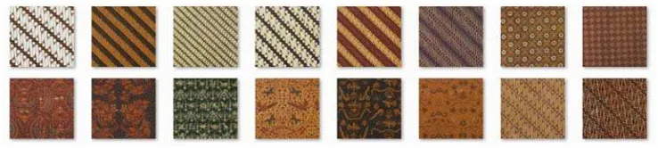
Batik image dataset is collected by capturing 50 types of batik fabric. Each fabric is captured to as much as six random images and then resized to 128x128 pixels size in JPEG format. Thus the total number of images in a dataset is 300 and consists of 50 classes. Examples of batik images are shown in Figure 1. In general, there are two patterns of captured batik images; geometric and non-geometric patterns.
Figure 1. Example of Batik images
3. Color Difference Histogram
CDH consists of five main sections. First, transforming an RGB image to L*a*b* color space. Second, detecting edge orientation and quantizing the values to m bins, m={6,12,18,24,30,36}. Third, quantizing each component of the image L*a*b* color into n bins, n={54,72,108}. Furthermore, calculating the difference of the color quantization and edge orientation map; and the difference of edge quantization and the color intensity map. Finally, combining the color histogram and edge orientation histogram.
3.1 RGB image to L*a*b* Color Space
RGB color space is a common color space that is used in general application. Though this color space is simple and straightforward, it cannot mimic human color perception. On the other side, L*a*b* color space was designed to be perceptually uniform [15], and highly uniform with respect to human color perception, thus L*a*b* color space is particularly a better choice in this case. In this section, we are transforming an RGB image to an XYZ color space before transforming to an L*a*b* color space.
3.2 Edge Orientation Detection in L*a*b* Color Space
is started by converting a color image to a grey-scale image. Then, gradient magnitude and orientation are detected based on the grey-scale image. However, this method suffers from the loss of a number of chromatic information.
To prevent the loss of chromatic information, we utilised the Zenzo [16] method to get the gradient from the color image. In this section, each L*a*b* component is detected with horizontal orientation (gxx) and vertical orientation (gyy), and then the computed dot product of gxx and gyy, resulting in gxy, using Sobel operators. Furthermore, the gradient consists of magnitude component and direction. In order to get the maximum rate of orientation change of gradient, the following formula is used:
, arctan (1)
Where the rate of orientation change for , given by equation (2) and (3)
, cos / (2)
, cos / / (3)
Moreover, we need to find the maximum value of gradient (Fmax)
max , (4)
Where:
,
, (5)
After computing the edge orientation for each pixel , , then we quantise the , into m bins, with variation m={6,12,18,24,30,36}. The interval size of each bin is calculated by dividing 360 with m. For example, for m=6, the interval size is 60, so all edge orientations are uniformly quantized to intervals of 0, 60, 120, 180, 240, 300.
3.3 Quantization L*a*b* Color Space
Color is one of the important aspects for image retrieval, because it provides highly reliable spatial information. This aspect is usually performed as features in a color histogram. Common applications typically use RGB color space for practical reasons, however, this cannot represent human visual perception.
Therefore, in this paper we use L*a*b* color space. Additionally, each component in L*a*b* is quantized to n bins, where n={54,63,72,81,90}. Given a color image of size M x N, for instance, if we set n=72, it is equal L=8, *a=3, *b=3.Denote by C(x,y) the quantized image, where 0<x<M,0<y<N.
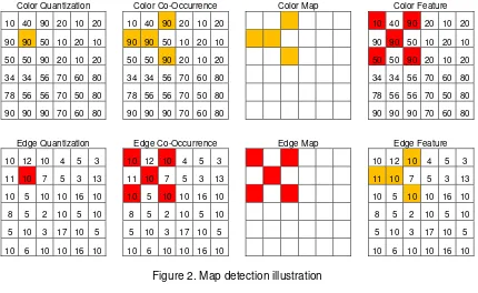
3.4 Map detection
are denoted by , and ′, ′ . For neighboring pixels, where the distance is D and respective quantization numbers for the color and edge orientations are W and V, we can define the color difference histogram as equation (6) and equation (7).
Color Quantization Color Co-Occurrence Color Map Color Feature
10 40 90 20 10 20 10 40 90 20 10 20 10 40 90 20 10 20
90 90 50 10 20 10 90 90 50 10 20 10 90 90 50 10 20 10
50 50 90 20 10 20 50 50 90 20 10 20 50 50 90 20 10 20
34 34 56 70 60 80 34 34 56 70 60 80 34 34 56 70 60 80
78 56 56 70 50 80 78 56 56 70 50 80 78 56 56 70 50 80
90 90 90 70 60 80 90 90 90 70 60 80 90 90 90 70 60 80
Edge Quantization Edge Co-Occurrence Edge Map Edge Feature
10 12 10 4 5 3 10 12 10 4 5 3 10 12 10 4 5 3
11 10 7 5 3 13 11 10 7 5 3 13 11 10 7 5 3 13
10 5 10 10 16 10 10 5 10 10 16 10 10 5 10 10 16 10
8 5 2 10 5 10 8 5 2 10 5 10 8 5 2 10 5 10
5 10 3 17 10 5 5 10 3 17 10 5 5 10 3 17 10 5
10 6 10 10 16 10 10 6 10 10 16 10 10 6 10 10 16 10
Figure 2. Map detection illustration
, ∑ ∆ ∆ ∆
, ′, ′ ; max | | , | | (6)
, ∑ ∆ ∆ ∆
, ′, ′ ; max | | , | | (7)
Where ∆ , ∆ and ∆ are difference value between two color pixels. In this paper we use D=1. If the edge orientation is W and quantization of color is V, then the feature of CDH denoted as follows:
, … , , … (8)
Where Hcolor is the color histogram and Hori is the edge orientation histogram. For instance, if we set the dimension of color quantization = 72 and edge orientation = 18, thus, the total features for image retrieval are 72 + 18 = 90 dimensional features. Furthermore, this total feature is denoted as H.
4. Gray Level Co-occurrence Matrix
normalizing the symmetrical matrix by computing the probability of each matrix element. Moreover, the final step is computing GLCM features. Each feature is computed by one distance pixel in four directions, those are 0°, 45°, 90° and 135°, to detect co-occurrence. When GLCM has a matrix with a size LxL, in which L is the number of gray levels of the original image and when the probability of pixel i is the neighbor of pixel j within distance d and edge orientation θ is P, the energy feature, the entropy feature, the contrast feature and the correlation feature can be calculated by equations (14), (15), (16) and (17).
∑, , , , (9)
∑, , , , . log , , , (10)
∑, . , , , (11)
∑, , , , (12)
Where ∑, . , , , , ∑, . , , , , ∑,
. , , ,
,
,
. , , ,
. Energy, also called as Angular Second Moment, is the representation of image homogeneity. When the value of energy is high, the relationships between pixels are highly homogenous. Entropy is the opposite of energy which represent the randomness value between images. A higher value of entropy indicates that the relations between pixels are highly random. Contrast is a variation of an image’s gray level. An image with a smooth texture has a low contrast value and an image with a rough texture has a high contrast value. Correlation is a linear relationship between pixels. Let, each GLCM feature 0°, 45°, 90° and 135° as Hasm(θ), Hent(θ), Hcont(θ), Hcorr(θ) where ∈ , ,9 , . So, the feature of GLCM is denoted as follows:° … ° , ° … ° , ° … ° ,
° . . . ° (13)
So, the final feature of a batik image is a combination of CDH features and GLCM features denoted as follows :
, (14)
For example, if we set the quantization of color = 72, it consists of R=8, G=3, B=3; quantization edge orientation = 18 and the total GLCM features are 16, so the total feature = 106.
5. Performance Measure
For each template image in the dataset, an M-dimensional feature vector T=[T1,T2,…TM] is extracted and stored in the database. Let Q=[Q1,Q2,…QM] be the feature
vector of a query image and the distance between them is simply calculated as
, ∑ | | | | | | (15)
Where ∑ and ∑ . The class labels of the template image that yield the smallest distance will be assigned to the query image.In this experiment, performance was measured using precision and recall which are defined as follows:
R(N) = IN / M (17)
WhereIN is the number of retrieved images, N is the number of relevant images, and M is the
number of all relevant data in the dataset.
6. Results and Discussion
Feature extraction using CDH results in 90 features which consist of 72 color features and 18 edge orientation features. Then, features extraction using GLCM results in 16 features which consist of features including energy, entropy, contrast and correlation. Each GLCM feature is computed in four directions, these are 0°, 45°, 90° and 135°. Totally, there are 106 features which can be represented on a histogram, as shown in Figure 3. Figure 3a is an example of a computed image with Figure 3b as its histogram representation. The horizontal axis represents 106 features, of which the first 72 features are color features, the second 18 features are edge orientation features and the last 16 are GLCM features. By utilizing these features, the similarity of images is computed using the Canberra based on equation (18); after which, the precision and the recall of the image retrieval process are computed based on equations (19) and (20). For evaluation purposes, one image is randomly selected from each class, resulting in 50 images as a data test. The evaluation is run to retrieve four, six and eight images based on each image in the data test. CDH, by default extracts 108 features which consist of 90 color features and 18 edge orientation features.
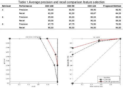
In this study, we varied the size of color quantization and feature quantization, and then combined the result with the GLCM features. The aim of this activity was to find the best quantization size such that the number of features is decreased while increasing precision at the same time. The evaluation is performed in four schemes. First, we use CDH with 108 features which consist of 90 color features (10x3x3) and 18 edge orientation features. Second, use CDH with 90 features which consist of 72 color features (8x3x3) and 18 edge orientation features. Third, use CDH and GLCM with 124 features which consist of 90 color features (10x3x3), 18 edge orientation features and 16 GLCM features. Finally, use CDH and GLCM with 106 features which consist of 72 color features (8x3x3), 18 edge orientation features and 16 GLCM features. The result is shown in Table 1. The average precision values for retrieving four, six and eight images in the four schemes are 81.92%, 81.53%, 85.44% and 85.44% respectively. The evaluation was conducted in Matlab 2013a and Windows 7 operation system with Core i5 2.3 Hz and 4 GB memory. The feature extraction of each image in each scheme took 1.091, 1.084, 1.097 and 1.086 seconds respectively. The result shows that the reduction of features from 108 to 90 may decrease precision by 0.39%. Though there is a lower precision, this difference is relatively small; on the opposite scale, a smaller number of features potentially decreases the complexity of the process.
(a) (b)
Figure 3. An example of Batik image and its histogram feature: (a) Batik image and (b) Histogram CDH of Batik image.
(a) (b) (c) (d) (e) Figure 4. An example of image retrieval: (a) The query image, (b-e) the similar images returned.
Table 1.Average precision and recall comparison feature selection
Retrieval Performance CDH 108 CDH 90 CDH 124 Proposed Method
4 Precision 93,00 93,50 95,50 96,50
Recall 62,00 62,33 63,67 64,33
6 Precision 85,00 83,33 90,33 89,33
Recall 85,00 83,33 90,33 89,33
8 Precision 67,75 67,75 70,50 70,50
Recall 90,33 90,33 94,00 94,00
Figure 5. The performance comparison of CDH and proposed method
0 50 100 150 200 250 300
7. Conclusion
This study presents image representation using a modified Color Difference Histogram and GLCM. The modification is performed in order to find the optimal color quantization size, so that the number of color features can be reduced. The reduced features, then, are replaced by GLCM features to improve image retrieval performance. Based on evaluation result, the proposed method is able to show higher precision when retrieving four images. The proposed method using 106 CDH features and 18 GLCM features, has 96.50% precision; whereas the use of 108 CDH features has 93.00% precision. The average precision of the proposed method when retrieving four, six and eight images is 3.85% higher than the original CDH. Therefore, we can conclude that the proposed method is able to perform better, while it has a smaller number of features compared to the original CDH for batik images retrieval.
References
[1] Fanani A, Yuniarti A, and Suciati N. Geometric Feature Extraction of Batik Image Using Cardinal Spline Curve Representation. TELKOMNIKA Telecommunication, Computing, Electronics and Control. 2014; 12(2).
[2] Minarno Agus-Eko, Munarko Yuda, Bimantoro Fitri, Kurniawardhani Arrie and Suciati Nanik. Batik Image Retrieval Based on Micro-Structure Descriptor. 2nd Asia-Pacific Conference on Computer Aided System Engineering–APCASE. Bali, Indonesia. 2014; 2: 63-64.
[3] Nugroho, Saptadi, and Darmawan U. Rotation Invariant Indexing For Image Using Zernike Moments and R-Tree. TELKOMNIKA Telecommunication, Computing, Electronics and Control. 2011; 9(2). [4] Li, Guizhi. Improving Relevance Feedback in Image Retrieval by Incorporating Unlabelled
Images. TELKOMNIKA Indonesian Journal of Electrical Engineering. 2013; 11(7): 3634-3640. [5] Zukuan, W. E. I., et al. An Efficient Content Based Image Retrieval Scheme. TELKOMNIKA
Indonesian Journal of Electrical Engineering. 2013; 11(11): 6986-6991.
[6] Irianto, Suhendro Y. Segmentation Technique for Image Indexing and Retrieval on Discrete Cosines Domain. TELKOMNIKA Telecommunication, Computing, Electronics and Control. 2012; 11(1): 119-126.
[7] RM Haralick, K Shangmugam, Dinstein. Textural feature for image classification. IEEE Transaction on Systems, Man and Cybermatics. 1973; SMC-2(6): 610-621.
[8] AK. Jain, A. Vailaya. Image retrieval using color and shape. Journal ofPattern Recognition. 1996; 29(8): 1233-1244.
[9] BS manjunath, JR. Ohm, VV. Vasudevan, A. Yamada. Color and texture descriptors. IEEE Conference on Circuit and Systems for video technology. 2001; 11(6): 703-715.
[10] B. Julesz, Textons. The elements of texture perception and their interactions. Nature. 1981; 290 (5802): 91-97.
[11] Guang-Hai Liu, Jing Yu Yang. Image Retrieval based on the texton co-occurrence matrix. Journal of Pattern Recognition. 2008;41: 3521-3527.
[12] Guang-Hai Liu, Lei Zhang, Ying-Kun Hou, Zuo Yong Li, Jing Yu Yang. Image Retrieval based on multi-texton histogram. Journal of Pattern Recognition. 2010; 43: 2380-2389.
[13] Guang-Hai Liu, Zuo-Yong Li, Lei Zhang, Yong Xu. 2011. Image Retrieval based on micro-structure descripor. Journal of Pattern Recognition. 2011; 44: 2123-2133.
[14] Guang-Hai Liu, Jing-Yu Yang. Content-based image retrieval using color difference histogram.
Journal of Pattern Recognition. 2013; 46: 188-198.
[15] RC. Gonzales, RE. Woods. Digital image processing. 3rd edition. Prentice Hall. 2007: 424:447. [16] SD Zenzo. A note on the gradient of multi image. Computer Vision, Graphic, and Image Processing.