DOI: 10.12928/TELKOMNIKA.v12i1.1706 87
Hierarchical Bayesian of ARMA Models Using
Simulated Annealing Algorithm
Suparman*1, Michel Doisy2 1
Department of Mathematical Education, University of Ahmad Dahlan, Jl. Prof. Dr. Soepomo, SH., Yogyakarta, Indonesia
2
ENSEEIHT/TESA, 2 Rue Camichel, Toulouse, France *Corresponding author, email: e-mail: [email protected]
Abstract
When the Autoregressive Moving Average (ARMA) model is fitted with real data, the actual value of the model order and the model parameter are often unknown. The goal of this paper is to find an estimator for the model order and the model parameter based on the data. In this paper, the model order identification and model parameter estimation is given in a hierarchical Bayesian framework. In this framework, the model order and model parameter are assumed to have prior distribution, which summarizes all the information available about the process. All the information about the characteristics of the model order and the model parameter are expressed in the posterior distribution. Probability determination of the model order and the model parameter requires the integration of the posterior distribution resulting. It is an operation which is very difficult to be solved analytically. Here the Simuated Annealing Reversible Jump Markov Chain Monte Carlo (MCMC) algorithm was developed to compute the required integration over the posterior distribution simulation. Methods developed are evaluated in simulation studies in a number of set of synthetic data and real data.
Keywords: Simulated Annealing, ARMA model, order identification, parameter estimation
1. Introduction
Suppose
x
1,
x
2,
,
x
n is a time series data. Time seriesx
1,
x
2,
,
x
n is said to be an ARMA
p
,
q
model, ifx
1,
x
2,
,
x
n satisfy following stochastic equation [3] :
t
x
z
qz
x
,
1 j
p
1 i i t i j
t j
t
t
1
,
2
,
,
n
(1)where
z
t is the random error at the time t,
i (i = 1, 2, ..., p) and
j (j = 1, 2, ..., q) is the coefficient-coefficient. Herez
t is assumed to have the normal distribution with mean 0 and variance
2. ARMA model
z t t
x
is called stationary if and only if the equality of polynomial1
pb
i0
i i
) p (
i
must lie outside the unit circle. Next ARMA model
z t tx
is called invertible if and only if the equality of polynomial
1
qb
j0
1 j
) q (
j
must lie outside the unit circle [4].
While for the order
p
,
q
is not known, the order identification and the parameters estimation are done in two stages. The first stage is to estimate the coefficients and error variance with the assumption of order
p
,
q
is known. Based on the parameter estimation in the first stage, the second stage is to identify the order
p
,
q
. A criterium used to determine order
p
,
q
has been proposed by many researchers, among others are the Akaike Information Criteria Criterion (AIC), Bayesian Information Criterion (BIC), and the Final Prediction Error Criterion (FPE).Based on the data
x
t,t
1
,
2
,
,
n
, this research proposes a method to estimate the valuep
,
q
,
(p),
(q), and
2 simultaneously. To do that, we will use a hierarchical Bayesian approach [10], which will be described below.2. Research Method 2.1 Hierarchical Bayesian
Let
s
x
pq1,
x
pq2,
,
x
n
be a realization of the ARMA
p
,
q
model. If the value
1 2 p q
0
x
,
x
,
,
x
s
is known, then the likelihood function ofs
can be written approximately as follows :
s
p
,
q
,
(p),
(q),
2
n 1 q p t ) q ( ) p ( 2 2 2 p n2
2
g
t
,
p
,
q
,
,
1
exp
2
1
(2)
where
q t j1 j ) q ( j i t p 1 i ) p ( i t ) q ( ) p (
z
x
x
,
,
q
,
p
,
t
g
fort
p
q
1
,
p
q
2
,
,
n
with initial value
x
1
x
2
x
pq
0
[11]. SupposeS
pandI
q are respectively stationary region and invertible region. By using the transformation
F
:
(p)
1(p),
2(p),
,
(pp)
S
p
p
p 2 1 ) p ()
1
,
1
r
,
,
r
,
r
r
(3)
(q)
q q ) q ( 2 ) q ( 1 ) q (I
,
,
,
:
G
q
p 2 1 ) q (
)
1
,
1
,
,
,
the ARMA model
x
t tz stationery if and only ifr
(p)
r
1,
r
2,
,
r
p
1
,
1
)
p
[2] and the ARMA model
x
t tz invertible if and only if
(q)
1,
2,
,
p
1
,
1
)
q
[1]. Then the likelihood function can be rewritten as:
s
p
,
q
,
r
(p),
(q),
2
n 1 q p t ) q ( 1 ) p ( 1 2 2 2 p n2
g
t
,
p
,
q
,
F
(
),
G
(
)
2
1
exp
2
1
(4)The prior distribution determination for parameters are as follows: a) Order p have Binomial distribution with parameters
:
max p(
1
)
pmax pp
p
p
max q(
1
)
qmax qq
q
q
c) Order p is known, the coefficient vectors
r
(p) have uniform distribution on the interval
p1
,
1
.d) Order q is known, the coefficient vectors
(q) have uniform distribution on the interval
q1
,
1
.e) Variance
2 have inverse gamma distribution with parameter2
and
2
:
2 1 2 22
2
2
exp
2
2
,
Here, the parameters
and
are assumed to have uniform distribution on the interval (0,1), the value of
is 2 and the parameters
is assumed have Jeffrey distribution. So the prior distribution for the parametersH
1
p
,
q
,
r
(p),
(q),
2
andH
2
,
can be expressed as:
H
1,
H
2
p
r
(p)p
q
(q)q
2
,
(5)According to Bayes theorems, then the a posteriori distribution for the parameters H1
and H2 can be expressed as:
H
1,
H
2s
s
H
1
H
1,
H
2
(6)A posteriori distribution is a combination of the likelihood function and prior distribution. The prior distribution is determined before the data is taken. The likelihood function is objective while this prior distribution is subjective. In this case, the a posteriori distribution
H
1,
H
2s
has the form of a very complex, so it can not be solved analytically. To handle this problem, reversible jump MCMC method is proposed.
2.2 Reversible Jump MCMC Method
Suppose
M
H
1,
H
2
. In general, the MCMC method is a method of sampling, as how to create a homogeneous Markov chain that meet aperiodic nature and irreducible ([9])m 2
1
,
M
,
,
M
M
to be considered such as a random variable following the distribution
H
1,
H
2s
. ThusM
1,
M
2,
,
M
m it can be used to estimate the parameter M. To realize this, the Gibbs Hybrid algorithm ([9]) is adopted, which consists of two phases:1. Simulation of the distribution
H
2H
1,
s
2. Simulation of the distribution
H
1H
2,
s
Gibbs algorithm is used to simulate the distribution
H
2H
1,
s
and the hybridused to simulate the distribution
H
1H
2,
s
. The reversible jump MCMC algorithm is generally of the Metropolis-Hastings algorithm [6], [8].2.2.1 Simulation of the distribution
H
2H
1,
s
The conditional distribution of H2 given (H1,s), writen
H
2H
1,
s
, can be expressed as
H
2H
1,
s
p(
1
)
pmaxp
q(
1
)
qmaxq2 2
2
exp
2
1
.
This distribution is inversion gamma distribution with parameters
2
and 2
2
1
. So the Gibbsalgorithm is used to simulate it.
2.2.2 Simulation of the distribution
H
1H
2,
s
If the conditional distribution of H1 given (H2, s), writen
H
1H
2,
s
, is integrated withrespect to
2, then we get
p
,
q
,
r
,
H
2,
s
) q ( ) p
(
22 1
H
,
s
d
H
Let
2
p
n
2
v
maxand
n
1 p t
) q ( ) p ( 1 2
max
G
)
r
(
F
,
q
,
p
,
t
g
2
1
2
w
and we use
2 v 2) v 1 ( 2
w
)
v
(
d
w
exp
then we get
p
,
q
,
r
,
H
2,
s
) q ( ) p
( max p pmax p
)
1
(
p
p
max q qmax q)
1
(
q
q
2
2
2
1
2 q p
1
v
w
)
v
(
On the other hand, we have also
2p
,
q
,
r
(p),
(q),
H
2,
s
2 (v 1)exp
w
2
So that we can express the distribution
H
1H
2,
s
as a result of multiplication of the distribution
p
,
q
,
r
,
H
2,
s
) q ( ) p
(
H
1H
2,
s
p
,
q
,
r
(p),
(q)H
2,
s
p
,
q
,
r
,
,
H
2,
s
) q ( ) p (
2
Next to simulate the distribution
H
1H
2,
s
, we use a hybrid algorithm that consists of two phases:• Phase 1: Simulate the distribution of
2p
,
q
,
r
(p),
(q),
H
2,
s
• Phase 2: Simulate the distribution
p
,
q
,
r
(p),
(q)H
2,
s
The Gibbs algorithm is used to simulate the distribution
2p
,
q
,
r
(p),
(q),
H
2,
s
.Conversely, the distribution
p
,
q
,
r
(p),
(q)H
2,
s
has a complex form. The reversible jumpMCMC is used to simulate it.
When the order
p
,
q
is determined, we can use the Metropolis Hastings algorithm. Therefore, in the case that this order is not known, Markov chain must jump from the order
p
,
q
with parameters
r
(p),
(q)
to the order
p
,
q
with the parameter
r
(p),
(q)
. To solve this problem, we use the Reversible Jump MCMC algorithm.2.2.3 Type of jump selection
Suppose
p
,
q
represent actual values for the order, we will write:
ARp the probability to jump from the p top
1
,
ARp the probability to jump from the p top
1
,
ARp the probability to jump from p to p,
MAq the probability to jump from q toq
1
,
MAq the probability to jump from the q toq
1
and
MAq the probability to jump from q to q. For each component, we will choose the uniform distribution on the possible jump. As an example for the AR, this distribution depends on p and satisfy
ARp
AR
p
1
AR
p
We set
AR0
AR0
0
and AR0
pmax
Under this restriction, the probability will be
)
p
(
)
1
p
(
,
1
min
c
AR
p and
)
1
p
(
)
p
(
,
1
min
c
AR p
with constant c, as much as possible so that
ARp
ARp
0
.
9
forp
0
,
1
,
,
p
max. The goal is to have
ARp
(
p
)
(
p
1
)
AR 1
p
2.2.4 Birth / Death of Order
As for the AR example, suppose that p is the actual value for the order of the ARMA model,
r
(p)
r
1,
r
2.
,
r
p
is the coefficient value. Consider that we want to jump from p to1
p
. We take the random variable u according to the triangular distribution with mean 0
1
u
0
,
u
1
We complete the vector
r
(p) random variables with u. So the new coefficient vector is proposed
r
,
r
.
,
r
,
u
r
1 2 p) 1 p (
Note that this transformation will change the total value of all. It is clearly seen that the Jacobian of the transformation of value is 1.
Instead, to jump from
p
1
to p is done by removing the last coefficients in
1 2 p p 1
) 1 p (
r
,
r
,
.
r
,
r
r
. So the new coefficient vectors that is proposed become
1 2 p
) p (
r
,
.
r
,
r
r
. The probability of acceptance / rejection respectively is
min
1
,
r
and
D
min
1
,
r
1where
s
,
H
,
r
,
q
,
p
s
,
H
,
r
,
q
,
1
p
r
2 ) q ( ) p ( 2 ) q ( ) 1 p (
(p) (p 1)
) p ( ) 1 p (
r
,
1
p
;
r
,
p
q
r
,
p
;
r
,
1
p
q
We have
)
r
(
g
r
,
1
p
;
r
,
p
q
r
,
p
;
r
,
1
p
q
1 p AR p ) 1 p ( ) p ( AR 1 p ) p ( ) 1 p (Finally, we get
(p) (q)
v( )) ( v ) q ( ) 1 p (
,
r
,
q
,
p
,
w
,
r
,
q
,
1
p
,
w
r
1
p
p
p
max
1
2
1
AR p AR 1 p
)
r
(
g
1
1 p2.2.5 Changes in coefficients
Suppose now that the AR part is selected to jump from p to p without a order change, but only the coefficient is changed . If
r
(p)
r
1,
r
2.
,
r
p
is the coefficient vector, we modify the coefficient vector. Consider thatr
1,
r
2,
,
r
p is courant point and supposing thatp 2 1
,
u
,
,
u
u
new point, we define the point ui in the following way:)
s
r
sin(
u
i
i
s
is taken with the uniform distribution on the interval
10
,
10
. Thenu
i is selected withthe distribution
2 i i iu
1
5
r
u
f
in the interval
)
10
r
sin(
),
10
r
If
r
(p)
r
1,
r
2.
,
r
i1,
r
i,
r
i1,
,
r
p
andr~
(p)
r
1,
r
2.
,
r
i1,
u
i,
r
i1,
,
r
p
, then the probability acceptance / rejection can be written by
C
min
1
,
r
CWhere
s
H
,
,
r~
,
q
,
p
s
H
,
,
r
,
q
,
p
r
2 ) q ( ) p ( 2 ) q ( ) p (C
(p) (p)
) p ( ) p (r
,
p
;
r~
,
p
q
r~
,
p
;
r
,
p
q
because
) p ( ) p ( ) p ( ) p (r
,
p
;
r~
,
p
q
r~
,
p
;
r
,
p
q
2 1 i i i iu
1
r
1
u
1
r
1
So
(p) (q)
v( )) ( v ) q ( ) p ( C
,
r
,
q
,
p
,
w
,
r
,
q
,
p
,
w
r
2 1 i i i iu
1
r
1
u
1
r
1
2.3 Simulated Annealing Algorithm
Simulated Annealing algorithm [7] is obtained by adding a line in the temperature
m 2
1
,
T
,
,
T
T
at the top of the MCMC method. Next simulated annealing algorithm will produce a Markov chainM
(
T
1),
M
(
T
2),
,
M
(
T
m)
which is no longer homogeneous. With ahypothetical on a certain
T
1,
T
2,
,
T
m [14] will be convergent to maximize the value of a posteriori distribution
H
1,
H
2s
.3. Results and Analysis
In As an illustration, we will apply this method to identify the order and estimate the parameter synthesis ARMA data and real ARMA data. Simulation studies are done to confirm that the performance of simulated annealing algorithm is able to work well. While case studies are given to exemplify the application of research in solving problems in everyday life.
For both synthesis ARMA data and real ARMA data, we will use the simulated annealing algorithm to identify order and estimate the parameters of the ARMA model. For this purpose, the simulated annealing algorithm is implemented for 70000 iterations with a value of initial temperature T0 = 10 and the temperature is derived with the temperature factor 0.995 up
to the end temperature T1400 = 0.01. Value of order p and q is limited to a maximum of 10. So
that
p
max
q
max
10
. [image:7.595.78.519.60.375.2]3.1 Synthetic ARMA data
Figure 1 shows a synthetic ARMA data. The data are made according to the equation (1) above, with the number of data n = 250, order p = 2, order q = 1,
(2)
1
.
36
,
0
.
7
,
0
.
7
) 1 (
Figure 1. ARMA Synthetic Data
Based on the synthetic data in Figure 1, next order p, q order, ARMA model parameter
and variance
2 are estimated by using the SA algorithm. The order p, q order, ARMA model parameter and variance
2 produced by the simulated annealing algorithm arepˆ
2
,qˆ
1
,
0
.
41
,
0
.
75
ˆ
(2)
,
ˆ
(1)
0
.
72
and
ˆ
2
1
.
06
. When we compare between the actual value and the estimator value, it shows that simulated annealing algorithm can work well.
3.2 Real ARMA Data
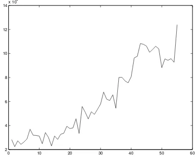
The real data in Figure 4 below is a passenger service charge (PSC) at the Adisutjipto International Airport in Yogyakarta Indonesia for the period 55 from January 2001 to July 2005.
Figure 2. First distinction of PSC data at the Adisutjipto International Airport Yogyakarta.
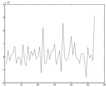
Clearly visible in Figure 4, the data are not stationary very day. To get stationary data the first distinction is made and the results shown in Figure 3.
0 50 100 150 200 250
−15 −10 −5 0 5 10 15
0 10 20 30 40 50 60
2 4 6 8 10 12 14x 10
[image:8.595.216.413.445.604.2]Figure 3. Second distinction of PSC data at the Adisutjipto International Airport.
Based on the data in Figure 3, next order p, q order, ARMA model parameter and variance are estimated by using the simulated annealing algorithm. The results are
pˆ
1
,0
qˆ
,
ˆ
(1)
0
.
38
dan
ˆ
2
6
.
75
10
7.4. Conclusion
The description above is a study of the theory of simulated annealing algorithms and its
application in the identification of order p and q, coefficient vectors estimation
(r) and
(q), and variance estimation
2 from the ARMA model. The results of the simulation show that the simulated annealing algorithm can estimate the parameters well. Simulated annealing algorithm can also be implemented with good results on Synthetic Aperture Radar image segmentation [13].As the implementation, the simulated annealing algorithm is applied to the PSC data at the Adisutjipto International Airport. Its result is that the PSC data can be modeled with the ARIMA model (1,0). The model can be used to predict the number of PSC at the Adisutjipto International Airport in the future.
References
[1] Barndorff-Nielsen O, and Schou G. On the parametrization of autoregressive models by partial autocorrelation. J. Multivar. Anal. 1973; 3: 408-419.
[2] Bhansali RJ. The inverse partial correlation function of a time series and its applications. J. Multivar.
Anal. 1983; 13: 310-327.
[3] Box GEP, Jenkins GM, Reinsel GC. Time Series Analysis: Forecasting and Control. New Jersey: Prentice Hall. 2013.
[4] Brockwell PJ, Davis RA. Times Series: Theory and Methods. Springer: New York. 2009.
[5] Green PJ. Reversible Jump Markov Chain Monte Carlo Computation and Bayesian model determination. Biometrika. 1995; 82: 711-732.
[6] Hastings WK. Monte Carlo sampling methods using Markov chains and their applications. Biometrika. 1970; 57: 97-109.
[7] Kirpatrick S. Optimization by Simulated Annealing: Quantitative Studies. Journal of Statistical Physics. 1984; 16:975-986.
[8] Metropolis N, Rosenbluth AW, Teller AH, and Teller E. Equations of state calculations by fast computing machines. Journal Chemical Physics. 1953; 21: 1087-1091.
[9] Robert CP. Méthodes de Monte Carlo par Chaînes de Markov. Economica. 1996.
[10] Robert CP. The Bayesian Choice. A Decision-Theoretic Motivation. Springer Texts in Statistics. 1994. [11] Shaarawy S, Broemeling L. Bayesian inferences and forecasts with moving averages processes.
0 10 20 30 40 50 60
−2 −1 0 1 2 3 4x 10
[12] Suparman, Soejoeti Z. Bayesian estimation of ARMA Time Series Models. WKSI Journal. 1999; 2(3): 91-98.
[13] Suparman. Segmentasi Bayesian Hierarki dalam Citra SAR dengan Menggunakan Algoritma SA.
Jurnal Pakar. 2005; 6: 227-235.
[14] Winkler G. Image Analysis, Random Fields and Dynamic Monte Carlo Methods : A Mathematical