Effect of outliers on estimators and tests in
covariance structure analysis
Ke-Hai Yuan*
Department of Psychology, University of North Texas, USA
Peter M. Bentler
Departments of Psychology and Statistics, University of California, Los Angeles, USA
A small proportion of outliers can distort the results based on classical procedures in covariance structure analysis. We look at the quantitative effect of outliers on estimators and test statistics based on normal theory maximum likelihood and the asymptotically distribution-free procedures. Even if a proposed structure is correct for the majority of the data in a sample, a small proportion of outliers leads to biased estimators and signi®cant test statistics. An especially unfortunate consequence is that the power to reject a model can be made arbitrarilyÐbut misleadinglyÐlarge by inclusion of outliers in an analysis.
1. Introduction
Covariance structure analysis (CSA) plays an important role in understanding the relationship among multivariate data (e.g. Bollen, 1989; Mueller, 1996). Letx1,. . .,xN be a sample of
dimensionpwithE(xi)5m, Cov(xi)5S, and let ÅxandSbe the sample mean vector and
sample covariance matrix. In CSA, S is ®tted by a structural model S5S(u) which hypothesizes the elements of the covariance matrix S to be functions of a more basic set of parameters u. The best-known example is the con®rmatory factor analysis model
S5LFL91W, where the unknown elements of the factor loading matrix L, the factor covariance matrix Fand the unique variance matrix Ware the elements ofu. In practice, covariance structure models S5S(u) often are rejected empirically. There are obviously many possible explanations for such empirical failures, all of which in some way must involve violation of regularity conditions associated with the theory on which the statistical tests are based. Of course, any particular modelS(u)may be inadequate, for example, it may omit crucial parameters or re¯ect an entirely incorrect functional form. Earlier technical development in this respect was given by Satorra & Saris (1985) and Steiger, Shapiro & Browne (1985), who proposed using the non-central chi-square to describe the distribution of the test statistics. Recent discussions of structural modelling imply that such theoretical
©2001 The British Psychological Society
inadequacy is almost inevitable in the social and behavioural sciences (de Leeuw, 1988; Browne & Cudeck, 1993).
In applications of structural equation models, the perspective that any model is only an approximation to reality dominates the literature. When a model does not ®t a data set as implied by a signi®cant chi-square test statistic, then many empirical researchers start using various ®t indices to justify their models (see, for example, Hu & Bentler, 1998). Some of them may go one step further to modify their models as facilitated by the modi®cation index in LISREL (JoÈreskog & SoÈrbom, 1993) or the Lagrange multiplier test in EQS (Bentler, 1995). This step was classi®ed as a model generating situation in JoÈreskog (1993). However, few or none of them question the quality of their data. This phenomenon was noted by Breckler (1990). JoÈreskog (1993) discussed various possible causes when a model does not match a data set in practice and emphasized the importance of proper data for proper statistical results. Even though there exist various approaches for outlier detection (Cook, 1986; Berkane & Bentler, 1988; Bollen, 1989; Bollen & Arminger, 1991; Tanaka, Watadani & Moon, 1991; Barnett & Lewis, 1994; Bentler, 1995; Cadigan, 1995; Fung & Kwan, 1995; Lee & Wang, 1996; Gnanadesikan, 1997; Kwan & Fung, 1998) as well as robust procedures (Huber, 1981; Hampel, Ronchetti, Rousseeuw & Stahel, 1986; Rousseeuw & van Zomeren, 1990; Wilcox, 1997; Yuan & Bentler, 1998a, 1998b; Yuan, Chan & Bentler, 2000), in the applications of CSA these techniques are seldom used as exempli®ed in numerous publi-cations using CSA in the applied journals in social and behavioural sciences (see, for example, MacCallum & Austin, 2000). This lack of attention to data quality probably occurs because there is no analytical development that directly connects the signi®cance of a chi-square test statistic to bad data. Such a development is one of the major foci of the current paper. Speci®cally, we will show that even if a proposed structure is correct for the majority of the data in a sample, a small proportion of outliers can lead to biased estimators and highly signi®cant test statistics.
Several approaches to CSA exist (Bollen, 1989). The two most widely used are the normal theory based maximum likelihood (ML) procedure and the asymptotically distribution-free (ADF) procedure (Browne, 1982, 1984). Of these two, the ML method is more popular among empirical researchers (Breckler, 1990). One reason for this is that the ML procedure is the default option in almost all the standard software (e.g., LISREL, EQS, AMOS). Another reason is that there exist various results about the robustness of the normal theory based ML procedure when applied to non-normal data (Browne, 1987; Shapiro, 1987; Anderson & Amemiya, 1988; Browne & Shapiro, 1988; Amemiya & Anderson, 1990; Satorra & Bentler, 1990, 1991; Mooijaart & Bentler, 1991; Satorra, 1992; Yuan & Bentler, 1999). The basic conclusion of this literature is that, under some special conditions, the parameter estimates based on ML are consistent, some standard errors remain consistent, and the likelihood ratio statistic can still follow a chi-square distribution asymptotically even when the observed data are non-normally distributed. The conditions under which normal theory methods can be applied to non-normal data are commonly referred to as asymptotic robustness conditions. Perhaps spurred on by a false sense of generalizability of the ML method, many researchers seldom bother to check the quality of their data. Once again, this phenomenon is probably due to the fact that there are no analytical results pointing out that asymptotic robustness is not enough when a data set contains outliers. As our results show, even if the observations in a sample come from normal distributions, the normal theory based ML still cannot verify the right covariance structure if there are a few outliers. Of course, the implication of the ADF
procedure is that whatever the distribution of a data set may be, this procedure will give a fair model evaluation when sample size is large enough. Unfortunately, the ADF method also can be distorted by a few outliers.
In the next section we will give the analytical results for the effect of outliers on the two commonly used procedures. In Section 3 we will use some real data sets as well as simulation to illustrate the effect of outliers in practice. Relatively technical proofs will be given in an appendix.
2. Effect of outliers on model evaluations
We will quantify the effect of outliers on the normal theory based ML procedure and on the ADF procedure. The following preliminaries will set up the framework for our study.
Letx1,. . .,xN0 come from a distribution G0,xN011,. . .,xN come from a distributionG1, N15N2N0andN0ÀN1. Let the mean vectors and covariance matrices ofG0andG1be m0 and m1, and S0 and S1, respectively. We will consider the structure S(u) such that S05S(u0)for some unknownu0, butS1will not equalS(u)for anyu. This means that we
have a correct covariance structure if there are no data from G1. Consequently, we will
consider theN1 cases as outliers in the CSA context. The above formulation is very general
because we do not put any speci®c distributional form onG1. For example, the commonly
used slippage model (see, Ferguson, 1961) for outlier identi®cation purposes is only a special case of the above model. When a variety of data contaminations exist in a sample,G1can be
regarded as a pooled distribution based on many sources of in¯uence (Beckman & Cook, 1983). We have no speci®c interest in identifying cases fromG1. The approach of in¯uence
analysis, as illustrated in Lee & Wang (1996) and Kwan & Fung (1998), should identify observations from G1, otherwise, a kind of Type I error is made in identifying the false
outliers.
In the above formulation, we assume thatN1is much smaller thanN0, and the memberships
of the observations are unknown. We may have knowledge about the impurity of the data, but we do not need to treatG1as another group. In practice, with observations from multiple
groups, the multiple-group approach (SoÈrbom, 1974) can be used to analyse the data when group membership is known, and a mixture distribution approach to structural modelling can be used when the group membership is unknown (Yung, 1997). Here, we have no special interest in the structure ofS1. The formulation is simply to study the quantitative effect of the
N1outliers on parameter estimators and test statistics. Since the ®nite-sample properties of
the estimators and test statistics are hard to quantify, we will concentrate on the large-sample properties.
We assume thatn0/nNp0andn1/nNp1asngrows large, wheren5N21,n05N021
andn15N121. Let ÅxandSbe the sample mean vector and the sample covariance matrix
based on the whole sample. It is easily seen that
Å
x¡¡N a.s.
m and S¡¡N a.s.
S , (1)
wherem 5p0m01p1m1and
S 5p0S01p1S11p0p1(m02m1)(m02m1)9. (2)
If we assumem05m1, thenS 5p0S01p1S1, but it may be unrealistic to assumeS0ÞS1
not be observed. IfS 5S(u )for someu , we can still recover the covariance structure, but the parameter is shifted with a bias ofu 2u0. However, because we usually do not observe
theu0, and chi-square statistics will not discriminateu fromu0, the effect of theN1outliers
will not be observed either. In the following, we will deal with the general case that
S05S(u0) butS1ÞS(u) for anyu. For the purpose of distribution characterization, we
will assume that the proportion of outliers is small so that estimates are still nearu0. Let
vech(·) be the operator which transforms a symmetric matrix into a vector by stacking the columns of the matrix, leaving out the elements above the diagonal. Let G5
Cov[vech{(x2m0)(x2m0)9}], wherex~ G0. For the distribution of s5vech(S), writing s5vech(S), we have the following lemma.
Lemma 2.1. If the ®rst four moments of bothG0andG1exist and are ®nite, then we
have:
(a) n p
(s2s0)NL Np(0,G)whenn1/
n p
N0;
(b) pn(s2s0)N L
Np(cg,G) when n1/
n p
Nc, where g5vech[S11(m02m1) (m02m1)92S0];
(c) pn(s2s0)NP `whengÞ0andn1/pnN`whilen1/nN0.
Lemma 2.1 tells us that the distribution ofpn(s2s0)varies as the proportion of out-liers changes. When the number of outout-liers is somewhere betweenpn andn, the quantity
n p
(s2s0)does not converge at all and hence standard statistical theory of CSA cannot be relied upon. For our purpose of quantifying the distribution of parameter estimates in CSA, we will be mainly interested in case (b), i.e.,n1/
n p
Nc.
In the rest of this paper, a dot on top of a function will denote the derivative (e.g., Ç
s(u)5 s(u)/u9). When a function is evaluated at u0, we sometimes omit its argument (e.g., Çs5s(u0)Ç ). We also need the following standard conditions for the results to be rigorous:
(C1) u0 is an interior point of some compact setQÌ q. (C2) S0 is positive de®nite andS(u)5S(u0)only whenu5u0.
(C3) S(u)is twice continuously differentiable. (C4) s(u)Ç is of full rank.
(C5) Gis positive de®nite.
Under the above conditions we will ®rst concentrate on the ML procedure and then turn to the ADF procedure.
2.1. Maximum likelihood procedure
Let S be the sample covariance based on a p-variate sample with size N5n11. The approach based on the normal theory ML procedure is to minimize
FML(S,S(u))5tr[SS2 1
(u)]2log|SS21(u)|2p (3)
for Ãu. LetDpbe the duplication matrix de®ned in Magnus & Neudecker (1988, p. 49) and W(u)5221D9p[S21(u)ÄS21(u)]Dp.
Under the assumption thatN150,G05Np (m0,S0), and the null hypothesis of a correct
hold. Readers who have interests in this direction are referred to Yuan & Bentler (1999) for a very general characterization.
Still assumingG05Np(m0,S0)andS05S(u0)for some unknownu0, our interest is in
the property of Ãuand TML whenN1 does not equal zero. The following lemma is on the
consistency of Ãuwhen the proportion of contaminated data is small.
Lemma 2.2. Under conditions (C1) and (C2), and ifn1/nN0, then Ãu¡¡N a,s
u0.
When the number of outliers is comparable with the sample size, the estimator Ãuwill no longer converge tou0; instead, Ãu¡¡N
a.s.
u0 which minimizesFML(S ,S(u)); we will not deal with this situation here. Sinceu0 is an interior point ofQ, whenn is large enough Ãuwill
satisfy
Ç
s9(u)W(à u)(sà 2s(u))à 50. (5)
For this Ãu, we have the following result.
Theorem 2.1. Under conditions (C3), (C4) and (C5), if ÃuNP u0, then:
Comparing with Lemma 2.1, Theorem 2.1 tells us that the asymptotic distribution of
(s2s0). The bias in the asymptotic distribution of n p
(uÃ2u0)will increase as the proportion of outliers increases. The non-centrality parameter (NCP) in the chi-square distribution, which characterizes the test statisticTMLas described in the following theorem,
will increase in a similar way.
(b) TMLN L
x2p2q(t)whenn1/
n p
Nc, where
t5c2g9[W2Ws(Ç sÇ9Ws)Ç 21sÇ9W]g. (6)
The NCP in (6) can be compared with the NCPs discussed in Satorra (1989) and Satorra, Saris & de Pijper (1991). Actually,tis just the W3 in Satorraet al.(1991) whenN15N,
c25n andg5O(1/pn). Notice that the assumption ofG05N(m0,S0) is used to obtain
simple expressions in Theorems 2.1 and 2.2. When G0 is not normal the bias in Ãu as an
estimator ofu0still exists. Similarly, even thoughTML cannot then be described by a
chi-square distribution, whenN1>0 it will be stochastically larger than whenN150.
2.2. The asymptotically distribution-free procedure
Since data sets in social and behavioural sciences may not follow multivariate normal distributions, Browne (1982, 1984) proposed the ADF procedure. Let yi5vech[(x12x)Å
(xi2x)Å 9]andSybe the sample covariance matrix ofyi. The ADF procedure is to minimize FADF(S,S(u))5(s2s(u))9S2y1(s2s(u)) (7)
for Äu. We do not need to assume a particular distribution to apply this procedure. Under the conditionsS05S(u0)andN150,
n p
(uÄ2u0)N L
N(0,Q), (8a)
whereQ5(sÇ9G21Ç s)21
and
TADF5nFADF(S,S(u))Ä N L
x2p2q. (8b)
Like the normal theory based ML procedure, the ADF procedure is also susceptible to poor data quality. Now, assuming thatS05S(u0)butN1 does not equal zero, we have the
following lemma.
Lemma 2.3. Under conditions (C1), (C2) and (C5), and ifn1/nN0, then Äu¡¡N a.s.
u0.
As in the previous subsection, we are interested in quantifying the effect of outliers on the distribution of Äuand on the test statisticTADF. To obtain Äu, we usually need to solve the
equation
Ç
s9(u)SÄ 2y1(s2s(u))Ä 50. (9)
The following theorem gives the asymptotic distribution of Äu.
Theorem 2.3. Under conditions (C3), (C4) and (C5), if ÄuNP u0, then:
(a) n p
(uÄ2u0)NL N(0,Q)whenn1/pnN0;
(b) n p
(uÄ2u0)NLN(w,Q)whenn1/pnNc, where
w5c(sÇ9G21Ç
s)21sÇ9G21 g;
Theorem 2.3 tells us that in the presence of outliers, the mean vector in the asymptotic distribution ofpn(uÄ2u0)will not be zero. It changes in a similar way to that for the ML
estimator. The bias in Äuin case (b) is mainly due to the effect of the outliers onS. Even though the outliers also affect the weight matrixS2y1, such an in¯uence on Äuis minimal. Actually, as
long asn1/napproaches zero,Sywill be consistent forG, which is suf®cient for the result in
the theorem to hold. The following theorem is on the corresponding test statistic.
Theorem 2.4. Under conditions (C3), (C4) and (C5), if ÄuNP u0, then:
(a) TADFN L
x2p2qwhenn1/
n p
N0;
(b) TADFN L
x2p2q(h)whenn1/
n p
Nc, where
h5c2g9[G212G21s(Ç sÇ9G21
Ç
s)21sÇ9G21 ]g.
It is obvious thatw5j andh5t whenG0 follows a multivariate normal distribution.
However, as we shall see in the next section, there may exist a big difference between the estimates by the two methods even whenN150.
From the results in this section, we can see the effect of outliers on the commonly used inference procedures. Even if a proposed model would ®t the population covariance matrix of G0, because of outliers, parameter estimates will be biased and test statistics will be
signi®cant. For example, in a factor analysis model, biased parameter estimates may lead to non-signi®cant factor loadings being signi®cant and vice versa (Yuan & Bentler, 1998a, 1998b), or there may even be an inability to minimize (2.3) or (2.7) using standard mini-mization methods. A signi®cant test statistic may discredit a theoretically correct model structureS05S(u0)that a researcher wants to recover (Yuan & Bentler, 1998b). As will be
illustrated in the next section, the NCP associated with a model test can be made larger for any actual degree of model misspeci®cation by inclusion of a few outliers. These outliers will seriously distort any power analysis that should be an integral part of structural modelling.
3. Illustration
We will ®rst use two data sets to demonstrate the relevance of our results to data analysis. In particular, we will show that a few outliers can create a problematic solution such as a Heywood case (negative error variance). The NCP estimate, on which most ®t indices are based, can also be strongly in¯uenced by outliers. Then we will conduct a simulation to see how the analytical results in Section 2 are matched with empirical data.
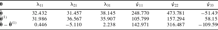
The ®rst example is based on a data set from Bollen (1989). It consists of three estimates of percentage cloud cover for 60 slides. This data set was introduced for outlier identi®-cation purposes. Bollen & Arminger (1991) further used a one-factor model to ®t this data set to study observational residuals in factor analysis. Fixing the factor variance at 1.0, the maximum likelihood solution Ãufor factor loadings and factor variances is given in the ®rst row of Table 1. With the negative variance estimates Ãw335251.439, this solution is
to the three largest residuals in Bollen & Arminger’s (1991) analysis, the solution Ãu(1)is given in the second row of Table 1. In this example, the outliers have a big effect on the estimates of error variances, but relatively less effect on the factor loadings.
For this example, the ADF procedure will give the same result as the ML procedure because the model is saturated. Notice that one has no way to evaluate the population parameterjorwbecause the true parameteru0is unknown. We may approximate the bias by
the parameter differences Ãu2uÃ(1), which is given in the third row of Table 1. Since the
degrees of freedom are zero, a test statistic is not relevant here.
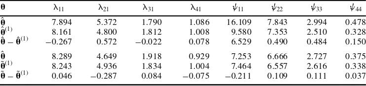
The second data set is from NBA descriptive statistics for 105 guards for the 1992±1993 basketball season (Chatterjee, Handcock & Simonoff, 1995). We select a subset of four variables from the original nine. These four variables are total minutes played, points scored per game, assists per game, and rebounds per game. Yuan & Bentler (1998a) proposed a one-factor model for these variables. Since the variable `total minutes played’ has a very large variance, as in Yuan & Bentler (1998a) it is multiplied by 0.01 before the model is ®tted. With factor varianceF51.0, the ML estimates based on the entire data set are given in the ®rst row of Table 2. The likelihood ratio statistic TML515.281, which is highly
signi®cant when referred tox22. This rejection of the model may be due to a few outlying
observations. Yuan & Bentler (1998a) identi®ed cases 2, 4, 6, 24, 32 as the ®ve most in¯uential cases. The model was re-estimated without these ®ve cases. The likelihood ratio statistic is nowTML54.918, which is not signi®cant at the 0.05 level. For this example, the
NCP estimate is 13.281 if based on the entire data set. This is more than four times its corresponding estimate, 2.918, when the ®ve cases are removed. As is well known, almost all popular ®t indices are based on the NCP estimate (see, for example, McDonald, 1989; Bentler, 1990). Hence, model evaluation using ®t indices without considering the in¯uence of outliers would be misleading. Similarly, power analysis without the ®ve in¯uential cases would lead to quite different conclusions about the one-factor model as compared to an analysis that would include these ®ve cases (e.g., Satorra & Saris, 1985). The new estimates Ã
u(1)as well as the approximate biases are given in the upper panel in Table 2. Even though the effect of the ®ve outliers on parameter estimates is not as deleterious as in the last example, some of the biases are not trivial.
The corresponding parameter estimates by the ADF approach are given in the lower panel of Table 2. The effect of the outliers on Äuis not as obvious as that on Ãu. However, their effect on the model evaluation also is dramatic. The test statistic based on the whole data set is TADF57.380, signi®cant at the 0.05 level, while the corresponding test without the ®ve
outlying cases is only 4.292. The NCP estimate based on the whole data set is more than twice of that based on the reduced data set.
While the effect of outliers can be seen in the two practical data sets, not knowing the true population parameters makes it impossible to evaluate how well the results in Section 2 match empirical research. To obtain better insight into this, we will conduct a simulation
K.-H. Yuan and P. M. Bentler 168
Table 1.Parameter estimates and biases for cloud cover data from Bollen (1989)
u l11 l21 l31 w11 w22 w33
Ã
u 32.432 31.457 38.145 248.770 473.781 251.439
Ã
u(1) 31.986 36.567 35.907 105.799 157.294 58.151
Ã
study. TheS0is generated by a one-factor model with ®ve indicators, that is,
S05L0L901W0,
whereL05(1.0,1.0,1.0,1.0,1.0)9andW05diag(0.5,0.5,0.5,0.5,0.5). TheS1is generated
by a two-factor model with
S15L1F1L911W1,
where
L15
1.0 1.0 0 0 0
0 0 1.0 1.0 1.0
© ª9
, F15
1.0 0.5
0.5 1.0
© ª
,
and W15diag(0.5,0.5,0.5,0.5,0.5). For the normal theory based method one needs to
chooseG05N5(m0,S0)in order for the chi-square approximation in Theorem 2.2 to hold.
Of course, other choices, such as a multivariatetdistribution, are legitimate forG1in the ML
method andG0 in the ADF method. A speci®c way of generating non-normal multivariate
distributions is as follows. Let A be a p3m (m$p) matrix such that AA95S1 and z5(z1,z2,. . .,zm)9, with zi being independent and Var(zi)51. Then x5Az5m1 will
have mean vectorm1and covariance matrixS1. For example, if one generatespindependent
chi-square variables (r1,r2,. . .,rp) each with two degrees of freedom, withzi5(ri22)/2,
thenx5S11/2z1m1will serve the purpose forx~ G1. Actually, it is not necessary to have
the distributional form of x speci®ed in such a way. More details for creating different multivariate non-normal distributions can be found in Yuan & Bentler (1999).
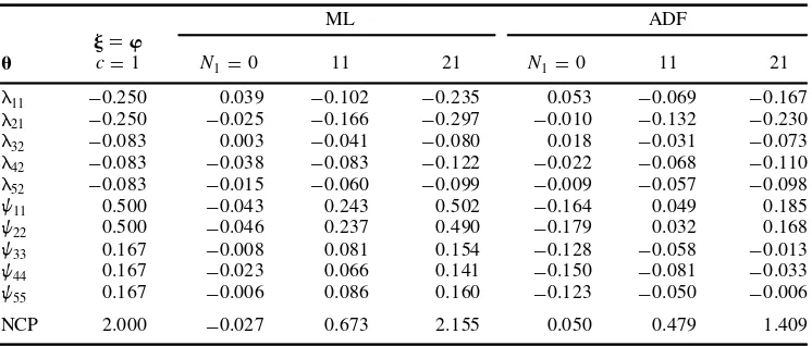
We chooseG05N5(0,S0)andG15N5(0,S1)in both the ML and the ADF procedures
for convenience. With such a design, j5w is easy to calculate and is given in the ®rst column in Table 3 forc51. With model degrees of freedomp 2q55 andt5h52.0 for c51, it is also easy for us to evaluate the NCP approximations given in Theorems 2.2 and 2.4. We choose sample sizeN5401,N1511 and 21, which lead toc<n1/
n p
50.5 and 1, respectively. For the purpose of comparison we also include the condition N150.
With 1000 replications the bias and NCP are calculated as
Bias5pn(uÅ2u0)
and
NCP5TÅ2df
respectively, where Åuand ÅTare the average of parameter estimates and test statistics across the 1000 replications.
Table 2.Parameter estimates and biases for NBA statistics data from Chatterjeeet al.(1995)
u l11 l21 l31 l41 w11 w22 w33 w44
Ã
u 7.894 5.372 1.790 1.086 16.109 7.843 2.994 0.478
Ã
u(1) 8.161 4.800 1.812 1.008 9.580 7.353 2.510 0.328
Ã
u2uÃ(1) 20.267 0.572 20.022 0.078 6.529 0.490 0.484 0.150 Ã
u 8.289 4.649 1.918 0.929 7.253 6.666 2.727 0.375
Ä
u(1) 8.243 4.936 1.834 1.004 7.464 6.557 2.616 0.338
Ä
WhenN1511 andc<1/2, the bias in Ãuin column 3 should be approximately half of the
theoretical ones underj5win column 1. Considering the ®nite-sample effect in column 2 when there is no theoretical bias, this approximation is pretty good. For example, instead of half of20.083, the bias forl42in column 3 is20.083. This may seem a bad approximation.
However, considering the random error20.038 in column 2, the amount that20.083 is off target just re¯ects the ®nite sample effect. With N521, the fourth column of numbers are estimates for the population numbers in column 1. Considering the ®nite-sample effect in column 2, the approximation is also quite good. With c<1/2, the theoretical NCPs are approximately 0.5 and 2.0, respectively. There exists some discrepancy between the NCP estimates and those theoretical NCPs. Similar discrepancies have been reported by Satorra et al.(1991), who studied various approximations to NCP whenN15Nandg5O(1/
n p
). In contrast to the bias approximations in the ML method, the bias approximations in the ADF procedure are substantially more off-target. This is related to the ®nite-sample effect, as shown in column 5, where there is no theoretical bias. This phenomenon was reported in Yuan & Bentler (1997a) under correct models, where the ®nite-sample bias in Äuis about 50 times of that for Ãu. Also, Äuis much less ef®cient than Ãuunless data are extremely non-normal. Considering these factors and comparing the last two columns of numbers under ADF with those forN150, we can see that the parameter estimates are shifted from those
correspond-ing to N150 by amounts roughly equal to w/2 and w, respectively. Similarly, the NCP
parameter estimate based on the ADF procedure is also some way off from the one described in Theorem 2.4. This may be related to the unstable nature ofTADF, as has been reported
previously (e.g., Yuan & Bentler, 1997b).
4. Discussion
We studied the effect of outliers on the two most commonly used CSA procedures. Even though a model structure may ®t the majority of the data, a few outliers can discredit the value of the model. The analytical development in Section 2 establishes a direct relation-ship between model statistical signi®cance and the presence of outliers. When a signi®cant chi-square statistic occurs in practice, the researcher should check the model as well as the
K.-H. Yuan and P. M. Bentler 170
Table 3.Simulation results on bias ( Åu2u0) and non-centrality parameter (T2df)
ML ADF
j5w
u c51 N150 11 21 N150 11 21
l11 20.250 0.039 20.102 20.235 0.053 20.069 20.167 l21 20.250 20.025 20.166 20.297 20.010 20.132 20.230 l32 20.083 0.003 20.041 20.080 0.018 20.031 20.073 l42 20.083 20.038 20.083 20.122 20.022 20.068 20.110 l52 20.083 20.015 20.060 20.099 20.009 20.057 20.098
w11 0.500 20.043 0.243 0.502 20.164 0.049 0.185
w22 0.500 20.046 0.237 0.490 20.179 0.032 0.168
w33 0.167 20.008 0.081 0.154 20.128 20.058 20.013 w44 0.167 20.023 0.066 0.141 20.150 20.081 20.033
w55 0.167 20.006 0.086 0.160 20.123 20.050 20.006
data since either could be the source of the lack of ®t. When data contain possible outliers, there are two general approaches to minimize their effect. One approach is to identify the outliers ®rst, and then to apply classical procedures after outlier removal (see, Lee & Wang, 1996). The other is to use a robust approach to downweight the in¯uence of outliers. With the ®rst approach, no method can guarantee that one can identify all the outliers. With the robust approach, the in¯uence of outliers is not necessarily completely removed. So the results in Section 2 may also be relevant to data analysis even when care has been taken to minimize the effect of outlying cases.
Our model formulation in Section 2 is for covariance structure analysis. We regard observations from G1 as outliers as long as u0 satis®es S05S(u0) while no u satis®es S15S(u). Thus, it is not necessary for outliers to be very extreme to break down the regular
analysis. A difference that characterizes our approach as compared to that of the robust statistic literature (e.g., regression), is that in robust statistics, it is usually assumed that the model is correct, but that error distributions have different tails. We assume here that the model is incorrect for the outliers. If a model is correct in both the means and covariances, the ADF procedure works well when sample size is large enough even though errors may have different third- and fourth-order moments (Yuan & Bentler, 1997b). Although outliers can have the effect of generating a sample that violates distributional assumptions in the ML procedure, this is not possible with the ADF procedure since it allows any distributional shape.
In the technical development in Section 2, we assumed n1/nN0 for convenience. In practice, sample sizes are always ®nite. WhenNÀN1, we can usec<n1/
n p
and the other corresponding sample quantities to approximate the biases in the normal distributions and non-centrality parameters in the chi-square distributions, as illustrated in the previous section. The proportion of outliers in a sample cannot be large in order for the asymptotic results in Section 2 to be a good approximation. This is parallel to the assumption
S05S(u )1O(1/
n p
)in Satorra & Saris (1985) and Steiger et al.(1985). These authors considered the behaviour ofTMLwhenN150.
One may not want to know details about outliers unless they are of special scienti®c interest. But outliers may in many instances represent important scienti®c opportunities to discover a new phenomenon. Potentially a new physical or theoretical aspect of a research area can be enriched by understanding the conditions and meaning associated with the occurrence of atypical observations. In such a case, focusing attention on only the majority of the data may be ignoring a fundamental and important phenomenon, and special scienti®c attention should be devoted to the analysis of atypical cases. Ultimately it may be possible to develop quite different models for various subsets of the data. In the case of covariance structure analysis, this is well known, and indeed multiple population models were developed primarily to deal with the case where a single model would distort a phenomenon. Our attention here is focused on the situation where prior research and theory dictate that a single multivariate process is at work and is of primary interest, and where there is recognition that subject carelessness, response errors, coding errors, transcribing problems or other unknown sources of distortion to a primary model may be operating, but are not of special interest. In this situation, we desire to quantify the effects that atypical observations may or may not have on a standard analysis.
all the asymptotic robustness research. The set-up in the asymptotic robustness literature assumes that a sample comes from a multivariate distribution whose covariance structure is of interest. Our set-up is that the majority of the data comes from a distribution withS05S(u0)
while a small proportion of outliers comes from a distribution that does not satisfy the proposed structural model. The implication of our result in this regard is that one should not misuse asymptotic robustness theory by blindly applying a model ®tting procedure in a CSA program to data with possible outliers.
Appendix
uniformly onQ. Since u0 minimizesFML(S0,S(u))and the model is identi®ed, the lemma
follows from a standard argument (Yuan, 1997). e
Proof of Theorem 2.1. Applying the ®rst-order Taylor expansion on the left-hand side of (5) atu0 gives
n p
(uÃ2u0)5(sÇ9Ws)Ç 21sÇ9Wpn(s2s0)1op(1). (A.3)
The theorem follows from Lemma 2.1 by noticing thatG5W21. e
Proof of Theorem 2.2. Using the Taylor expansion on FML(s)5FML(S,S(u))Ã at
It follows from (A.3) that
Putting (A.6) into (A.5), one obtains
TML5e9Qe1op(1), (A.7)
21. Noticing thatQis a projection matrix of rankp
2q, the
theorem follows from Lemma 2.1 and (A.7). e
Proof of Lemma 2.3. This is similar to the proof of Lemma 2.2.
Proof of Lemma 2.3. Using the Taylor expansion ofs(u)in (2.9) atu0, it follows that
Proof of Theorem 2.4. We have from (A.8),
The authors gratefully acknowledge the constructive comments of three referees and the editor that led to an improved version of the paper. This work was supported by National Institute on Drug Abuse grants DA01070 and DA00017 at the US National Institutes of Health.
References
Anderson, T. W., & Amemiya, Y. (1988). The asymptotic normal distribution of estimators in factor analysis under general conditions.Annals of Statistics,16, 759±771.
Barnett, V., & Lewis, T. (1994).Outliers in statistical data(3rd ed.). Chichester: Wiley.
Beckman, R. J., & Cook, R. D. (1983).Outlier . . . .s (with discussion).Technometrics,25, 119±163. Bentler, P. M. (1990). Comparative ®t indexes in structural models. Psychological Bulletin, 107,
238±246.
Bentler, P. M. (1995).EQS structural equations program manual. Encino, CA: Multivariate Software. Berkane, M., & Bentler, P. M. (1988). Estimation of contamination parameters and identi®cation of
outliers in multivariate data.Sociological Methods and Research,17, 55±64. Bollen, K. A. (1989).Structural equations with latent variables. New York: Wiley.
Bollen, K. A., & Arminger, G. (1991). Observational residuals in factor analysis and structural equation models.Sociological Methodology,21, 235±262.
Breckler, S. J. (1990). Application of covariance structure modeling in psychology: Cause for concern? Psychological Bulletin,107, 260±273.
Browne, M. W. (1982). Covariance structure analysis. In D. M. Hawkins (Ed.),Topics in applied multivariate analysis(pp. 72±141). Cambridge: Cambridge University Press.
Browne, M. W. (1984). Asymptotic distribution-free methods for the analysis of covariance structures. British Journal of Mathematical and Statistical Psychology,37, 62±83.
Browne, M. W. (1987). Robustness of statistical inference in factor analysis and related models. Biometrika,74, 375±384.
Browne, M. W., & Cudeck, R. (1993). Alternatives ways of assessing model ®t. In K. A. Bollen & J. S. Long (Eds.),Testing structural equation models(pp. 136±162). Newbury Park, CA: Sage. Browne, M. W., & Shapiro, A. (1988). Robustness of normal theory methods in the analysis of linear latent variate models.British Journal of Mathematical and Statistical Psychology,41, 193±208. Cadigan, N. G. (1995). Local in¯uence in structural equation models.Structural Equation Modeling,2,
13±30.
Chatterjee, S., Handcock, M. S., & Simonoff, J. S. (1995).A casebook for a rst course in statistics and data analysis. New York: Wiley.
Cook, R. D. (1986). Assessment of local in¯uence (with discussion).Journal of the Royal Statistical Society, Series B,48, 133±169.
de Leeuw, J. (1988). Multivariate analysis with linearizable regressions.Psychometrika,53, 437±455. Ferguson, T. S. (1961). On the rejection of outliers. In J. Neyman (Ed.),Proceedings of the fourth Berkeley symposium on mathematical statistics and probability, Vol. 1 (pp. 253±297). Berkeley: University of California Press.
Fung, W. K., & Kwan, C. W. (1995). Sensitivity analysis in factor analysis: Difference between using covariance and correlation matrices.Psychometrika,60, 607±614.
Gnanadesikan, R. (1997).Methods for statistical data analysis of multivariate observations(2nd ed.). New York: Wiley.
Hampel, F. R., Ronchetti, E. M., Rousseeuw, P. J., & Stahel, W. A. (1986).Robust statistics: The approach based on inuence functions. New York: Wiley.
Hu, L., & Bentler, P. M. (1998). Fit indices in covariance structural equation modeling: Sensitivity to underparameterized model misspeci®cation.Psychological Method,3, 424±453.
Huber, P. J. (1981).Robust statistics. New York: Wiley.
JoÈreskog, K. G. (1993). Test structural equation models. In K. A. Bollen & J. S. Long (Eds.),Testing structural equation models(pp. 294±316). Newbury Park, CA: Sage.
JoÈreskog, K. G., & SoÈrbom, D. (1993).LISREL 8 user’s reference guide, Chicago: Scienti®c Software International.
Kwan, C. W., & Fung, W. K. (1998). Assessing local in¯uence for speci®c restricted likelihood: Application to factor analysis.Psychometrika,63, 35±46.
Lee, S.-Y., & Wang, S.-J. (1996). Sensitivity analysis of structural equation models.Psychometrika,61, 93±108.
MacCallum, R. C., & Austin, J. T. (2000). Applications of structural equation modeling in psycho-logical research.Annual Review of Psychology,51, 201±226.
Magnus, J. R., & Neudecker, H. (1988).Matrix differential calculus with applications in statistics and econometrics. New York: Wiley.
McDonald, R. P. (1989). An index of goodness-of-®t based on noncentrality.Journal of Classication, 6, 97±103.
Mooijaart, A., & Bentler, P. M. (1991). Robustness of normal theory statistics in structural equation models.Statistica Neerlandica,45, 159±171.
Mueller, R. O. (1996).Basic principles of structural equation modeling.New York: Springer-Verlag. Rousseeuw, P. J., & van Zomeren, B. C. (1990). Unmasking multivariate outliers and leverage points
(with discussion).Journal of the American Statistical Association,85, 633±651.
Satorra, A. (1989). Alternative test criteria in covariance structure analysis: A uni®ed approach. Psychometrika,54, 131±151.
Satorra, A. (1992). Asymptotic robust inferences in the analysis of mean and covariance structures. Sociological Methodology,22, 249±278.
Satorra, A., & Bentler, P. M. (1990). Model conditions for asymptotic robustness in the analysis of linear relations.Computational Statistics & Data Analysis,10, 235±249.
Satorra, A., & Bentler, P. M. (1991). Goodness-of-®t test under IV estimation: Asymptotic robustness of a NT test statistic. In R. GutieÂrrez & M. J. Valderrama (Eds.),Applied stochastic models and data analysis(pp. 555±567). Singapore: World Scienti®c.
Satorra, A., & Saris, W. E. (1985). Power of the likelihood ratio test in covariance structure analysis. Psychometrika,50, 83±90.
Satorra, A., Saris, W. E., & de Pijper, W. M. (1991). A comparison of several approximations to the power function of the likelihood ratio test in covariance structure analysis.Statistica Neerlan-dica,45, 173±185.
Shapiro, A. (1987). Robustness properties of the MDF analysis of moment structures.South African Statistical Journal,21, 39±62.
SoÈrbom, D. (1974). A general method for studying differences in factor means and factor structure between groups.British Journal of Mathematical and Statistical Psychology,27, 229±239. Steiger, J. H., Shapiro, A., & Browne, M. W. (1985). On the multivariate asymptotic distribution of
sequential chi-square statistics.Psychometrika,50, 253±264.
Tanaka, Y., Watadani, S., & Moon, S. H. (1991). In¯uence in covariance structure analysis: With an application to con®rmatory factor analysis. Communication in Statistics—Theory and Methods,20, 3805±3821.
Wilcox, R. R. (1997).Introduction to robust estimation and hypothesis testing. San Diego: Academic Press.
Yuan, K.-H. (1997). A theorem on uniform convergence of stochastic functions with applications. Journal of Multivariate Analysis,62, 100±109.
Yuan, K.-H., & Bentler, P. M. (1997a). Improving parameter tests in covariance structure analysis. Computational Statistics and Data Analysis,26, 177± 198.
Yuan, K.-H., & Bentler, P. M. (1997b). Mean and covariance structure analysis: Theoretical and practical improvements.Journal of the American Statistical Association,92, 767±774. Yuan, K.-H., & Bentler, P. M. (1998a). Robust mean and covariance structure analysis.British Journal
of Mathematical and Statistical Psychology,51, 63±88.
Yuan, K.-H., & Bentler, P. M. (1998b). Structural equation modeling with robust covariances. Sociological Methodology,28, 363±396.
Yuan, K.-H., & Bentler, P. M. (1999). On normal theory and associated test statistics in covariance structure analysis under two classes of nonnormal distributions.Statistica Sinica,9, 831± 853. Yuan, K.-H., Chan, W., & Bentler, P. M. (2000). Robust transformation with applications to structural
equation modelling.British Journal of Mathematical and Statistical Psychology,53, 31±50. Yung, Y.-F. (1997). Finite mixtures in con®rmatory factor analysis models. Psychometrika, 62,
297±330.