FEATURE SELECTION AND PARAMETER OPTIMIZATION WITH
GA-LSSVM IN ELECTRICITY PRICE FORECASTING
Intan Azmira, W.A.R
Universiti Teknikal Malaysia Melaka, Malacca, Malaysia & National Energy University, Selangor, Malaysia, +606-555 2355, +606-555 2222, [email protected]
Izham, Z.A
National Energy University, Selangor, Malaysia, +603-89212020, Izham@uniten,edu.my
Keem Siah, Y.
National Energy University, Selangor, Malaysia, +603-89287309, yapkeem@uniten,edu.my
Titik Khawa, A.R.
King Abdulaziz University, Jeddah, Saudi Arabia, 6952000 012, [email protected]
Abstract. Forecasting price has now become essential task in the operation of electrical power system. Power producers and customers use short term price forecasts to manage and plan for bidding approaches, and hence
increasing the utility’s profit and energy efficiency as
well. The main challenge in forecasting electricity price is when dealing with non-stationary and high volatile price series. Some of the factors influencing this volatility are load behavior, weather, fuel price and transaction of import and export due to long term contract. This paper proposes the use of Least Square Support Vector Machine (LSSVM) with Genetic Algorithm (GA) optimization technique to predict daily electricity prices in Ontario. The selection of input data
and LSSVM’s parameter held by GA are proven to
improve accuracy as well as efficiency of prediction. A comparative study of proposed approach with other techniques and previous research was conducted in term of forecast accuracy, where the results indicate that (1) the LSSVM with GA outperforms other methods of LSSVM and Neural Network (NN), (2) the optimization algorithm of GA gives better accuracy than Particle Swarm Optimization (PSO) and cross validation. However, future study should emphasize on improving forecast accuracy during spike event since Ontario power market is reported as among the most volatile market worldwide.
Key words: Electricity Price forecasting, Least
Square Support Vector Machine (LSSVM), Genetic Algorithm (GA), Particle Swarm Optimization (PSO)
1. Introduction
In deregulated electricity market, forecasting electricity price is more challenging compared to predicting the load or demand [1] due to the volatility of price series with unexpected price spikes at any point of series. Sudden disruption at generation and transmission sites, imbalance between supply and demand, as well as weather condition, are the common factors influencing fluctuation in price series. Other aspects may also affect price series, such as bidding policy and operating reserve price [2]. Therefore, many methods have been explored by previous researchers to forecast electricity price. Time series models have been proven able to give satisfactory result [2]–[6] for stable market, but generally they are more appropriate for linear problem whilst price series is a non-linear pattern.
examples including noises and outliers rather than catching the relationship between input and output.
Hence, generalization problem often occurs where the developed model cannot predict well with the presence of unseen data during testing phase; consequently producing large error. Meanwhile, neural network usually spends more time during training process, especially when more training data, hidden neuron and hidden layer are added [17]. In addition, the prediction accuracy may be unstable or change for each run of simulation.
Support vector machine is another technique which has been reported as a better method than time series [20] and neural network [1]–[4], [21]– [31] in terms of model complexity, accuracy and efficiency. In [32], Chaotic Least Squares Support Vector Machine (CLSSVM) was combined with Wavelet Transform (WT) and Exponential Generalized Autoregressive Conditional Heteroskedastic (EGARCH) model to handle high volatility price series with the average error of 2.7% for PJM market and 2.58% for Spanish market. The hybrid method of rolling time series and LSSVM yielded MAPE of 2.26%; outperforming BPNN (4.11%) and ARMAX-AR-GARCH (2.72%) in [3]. Same goes for GA-LSSVM method in [26] method which produced MAPE of 4.2-9.7%; surpassing other techniques for all seasons.
On the other hand, the inclusion of optimization approach could improve the performance of forecasting. Literature in [33] applied modified relief and mutual induction to select input feature, and yielded MAPE of 4.55% (PJM), 5.22% (Spanish) and 17-19% (Ontario). Meanwhile, Modified Levenberg Marquardt with fuzzy c-mean (FCM) was applied to group daily load in [11], producing MAPE of 5.5-8.4% when applying Correlation Analysis for feature selection. Other literatures applied mutual information (MI) and Discrete Wavelet Transform (DWT) techniques for feature selection and Chaotic Gravitational Search Algorithm (CGSA) to reduce Gaussian noise and find the parameters of LSSVM [34], correlation analysis as feature selection and PSO as parameter selection of LSSVM [35], Self-Organizing Map (SOM Neural Network) to group data according to their similarities and PSO as parameter selection of LSSVM [1], correlation analysis as feature inspired Particles Swarm Optimization (QPSO) for similar day method [38], Rough Set as data selection and PSO as parameter selection of SVM [29], Principal Component Analysis (PCA) and K-Nearest Neighbor (KNN) as data selection [22], GA to select parameters for SVM [25] and LSSVM’s parameters [39], [26] Artificial Fish Swarm Algorithm (AFSA) [28] and Independent Component Analysis (ICA) as feature selection [27].
2. Fundamental of SVM, LSSVM, GA and PSO
This section introduces the fundamental of SVM, LSSVM, GA and PSO in terms of their theories and concepts.
2.1 SVM and LSSVM
Support Vector Machine (SVM) as presented by Vapnik [40] is a supervised learning model that supports data analysis and pattern recognition for classification and estimation.
Assume that an empirical data is set as
( 1, 1),....,( , )
;patterns. For linear functions
f,
Support Vector Regression functions to solve
for quadratic programs with
ɛ
-insensitive loss
function which involves inequality constraint.
Hence, SVM has high computational problem
where the optimization problem is defined as
while the ɛ-insensitive loss function is defined as
Thus, Least Squares Support Vector Machines (LSSVM) as suggested by Suykens and Vandewalle [41] can be used to solve this problem with linear Karush-Kuhn Tucker (KKT) equations, instead of using quadratic programming approach. The optimization problem is then denoted as
k k k
regularization constant that limits the trade-off between the fitting error minimization and smoothness of the estimated function [42]. The Lagrangian is defined as
}
where αiϵ R are the Lagrange multipliers; agreeing
to Wolfe’s duality theory. The αi in SVM is
positive but it may be negative or positive for LSSVM [43]. Hence, by using equality instead of inequality constraints, the LSSVM representation for estimation is developed as
b function. Therefore, LSSVM is less complicated [41], [44], more robust for more complex data and more efficient than SVM [43], [45]. The parameters
for SVM usually involves C, ɛ and σ, while LSSVM has only σ and γ [4], [25], [30], [32], [46].
2.2Genetic Algorithm (GA)
Genetic algorithm (GA) is one of Evolutionary Algorithms (EA) approaches, where the optimization approaches are based on population [47]. EA has common processes of mutation, crossover, natural selection, reproduction and
recombination [48]. Other methods in EA family are Evolution Strategy (ES), Genetic Programming (GP) and Evolutionary Programming (EP). In a GA, a population of candidate solutions, which is known as individuals or creatures, should have a set of chromosomes for each of candidate solution. The chromosomes can be mutated and changed. Usually, the solutions are denoted as a binary string which is 0 or 1, but other encodings are also permitted [49].
Typically, the evolution begins by generating random individuals from a population, where at each phase, individuals are randomly chosen as parents. Children are then produced and the processes are repeated. Consequently, an ideal solution is achieved and the fitness of every individual in each generation is calculated. The fitness is an objective function that is used to measure the performance of each chromosome. In this study, the fitness function is represented Mean Absolute Percentage Error (MAPE). The algorithm is usually terminated when the generation reaches its maximum value or an acceptable fitness value is obtained. Second generation population is then generated from the selected solutions, where normally a new solution
imitates many of its parent’s characteristics.
2.3 Particle Swarm Optimization (PSO)
Particle Swarm Optimization (PSO) was introduced by James Kennedy and Russell Eberhart. PSO mimicks the social behavior of a group of approach the same location. The best fitness with the best co-ordinate for each particle is called as personal best, pbest. Meanwhile, each particle also gets to know the fitness of those in its neighborhood and uses the position or gbest of the ones with the best fitness to adjust the particle’s velocity. Hence, the new position for each particle is its old position plus the new velocity or as following equation:
where vidk and xidk are the velocity of particle i at k
times and the position, respectively, pbestidk is the position of individual i at its best position at k times, gbestdk is the position of the group at the best position. The speed of the particle is capped to
–vdmax and vdmax to limit the searching space. c1 and
c2 denote the speeding figure that can adjust the
velocity of the particle [50], while r1 and r2
represent random fiction.
3. Research Design
This section discusses the selection of input data and accuracy measure. The inputs were chosen based on significant impact on price forecasting that had strong correlation with price characteristics.
3.1 Input Selection and Data Normalization
Data from 10–23 January 2010 of Ontario power market; two weeks prior to the testing period, was selected as the training data with 74 input features which comprised of:
1. the maximum load on the day before target day; Lmax(d-1)
2. day type of target day (-1 for weekend and 1 for weekday)
3. 24-hour loads on target day
4. 24-hour Hourly Ontario Electricity Price (HOEP)(s) on the day before target day 5. 24-hour generation’s prices on the day
before target day
Fig. 1: HOEP of 10–23 January 2010 for training purpose
Figure 1 shows the HOEP series used for training purpose. The testing data was selected from 25–31 January 2010. The training and testing data were normalized to prevent the domination of very large value in the data [2]. The data was normalized between [-1, 1] as in formula (9):
2 2
min max
min max
x x
x x x x
j
n (9)
where xn is normalized value, xj is the raw sample
value, xmax and xmin are the maximum and
minimum value of each feature in the samples.
3.2 Error Evaluation Function
Weekly Mean Absolute Percentage Error (WMAPE), Weekly Mean Absolute Error (WMAE) and regression value (R) were applied to measure the performance of forecast results. Regression value measures the correlation between actual value was used to measure the correlation between the actual value and forecast value as the closest value of 1, indicating strong correlation where the forecast result was able to follow the actual value very closely. The MAPE and MAE formulas were defined as:
N
t a ctua lt
foreca st t
a ctua l
P P P
N
MAPE t
1
100
(10)
N
t
foreca st t
a ctua l P t
P N MAE
1
1
(11)
where Pactual and Pforecast are the actual and forecast
HOEP at hour t, respectively, while N is the number of hours in a week.
4. Results and Discussion
This section presents the simulation results of LSSVM and Neural Network. All simulations were held in Matlab. LSSVMlab was chosen as LSSVM
0 20 40 60 80 100 120 140 160 10
20 30 40 50 60 70 80 90 100 110
Hour
H
O
E
P
(
$
/M
W
h
)
X: 130 Y: 104.2
Actual HOEP Prediction of LSSVM
compared with the stand alone LSSVM. The Neural Network model was also being compared with the LSSVM models to prove the accuracy of LSSVM.
4.1 LSSVM
Cross validation technique was applied to search the gamma (γ), and sigma (σ) values. The range of searching was set for [exponential (-25, 25)] for both gamma and sigma. Table 1 shows some of the LSSVM’s results when using cross validation for different values of gamma and sigma. The best MAPE was found to be 13.0871% when gamma=2 and sigma=32. Table 2 shows the simulation time was 1.56 minutes while the regression (R) was 0.478.
Table 1: MAPE for LSSVM
Gamma (γ)
Sigma
(σ) 21 21 23 24 25
21 13.1256 13.1928 13.2808 13.5880 14.0289 22 13.2864 13.4042 13.5569 13.7386 13.9808
23 13.3012 13.5097 13.7608 14.1209 14.5080 24 13.1851 13.4071 13.7067 14.0907 14.5762
25 13.0871 13.2155 13.4808 13.8542 14.3294
Table 2: Forecast accuracy measures of LSSVM, LSSVM-GA, LSSVM-PSO and NN
Model Selected input WMAPE WMAE
Simulation time (minutes)
Regression (R)
LSSVM all 74
inputs 13.0871 5.6575 1.5567 0.4780
LSSVM-GA 31 10.6072 4.3801 20.1895 0.7651
LSSVM-PSO 31 10.8019 4.3989 20.2592 0.7643
Neural Network
all 74
inputs 15.7813 6.8281 1.4853 0.3943
4.2 LSSVM with GA and PSO
Genetic Algorithm and Particle swarm optimization (PSO) were applied to select significant input features and the parameters for LSSVM. The population size and generation were fixed to 100 and 300, respectively, for both GA and PSO. The crossover fraction for GA was 0.5, while each of the two parameters of LSSVM was represented by ten bits. The result in Table 2 shows that only 31 inputs were selected for LSSVM-GA and LSSVM-PSO compared to 74 inputs for
LSSVM and NN. The gamma and sigma for GA were 24.7851 and 164.0292, while the gamma and sigma for PSO were 55.0387 and 293.2622. The selected inputs were:
HOEP at hour 9, 11, 12, 14, 18, 20 and 21 on the day before target day
Forecast load at hour 1-20 on target day Generation’s price at hour 1, 4, 6 and 19
on the day before target day
It was observed that LSSVM-GA performed better than LSSVM-PSO and other models in terms of WMAPE, WMAE and regression (R). In fact, the result achieved was better than that of proposed model in [38] for the same market model and test period. The average MAPEs for the three cases in [38] were 11.79% (SVM-GA), 11.98% (SVM-PSO) and 11.11% (SVM-QPSO; Quantum Inspired Particles Swarm Optimization QPSO).
4.3 Neural Network
A neural network model (NN) was developed to compare the performance of LSSVM and NN. Three layers were applied for the NN model, which consisted of an input layer, a hidden layer with a hidden neuron and an output layer. All 74 inputs were fed into the input layer, where no feature selection was held. The output layer produced 24 outputs representing 24 hours. Tansig and purelin transfer function were used for hidden and output layer, respectively. Similar cross validation procedure as for LSSVM was performed to select the number of hidden neuron in the hidden layer. Table 2 shows that NN model produced the least of MAPE and MAE, at 15.7813% and 6.8281, respectively.
0 20 40 60 80 100 120 140 160 10
20 30 40 50 60 70 80 90 100 110
Hour
H
O
E
P
(
$
/M
W
h
)
Actual HOEP Prediction of LSSVM-PSO
0 20 40 60 80 100 120 140 160 10
20 30 40 50 60 70 80 90 100 110
Hour
H
O
E
P
(
$
/M
W
h
)
Actual HOEP Prediction of Neural Network
0 20 40 60 80 100 120 140 160 10
20 30 40 50 60 70 80 90 100 110
Hour
H
O
E
P
(
$
/M
W
h
)
Actual HOEP Prediction of LSSVM-GA
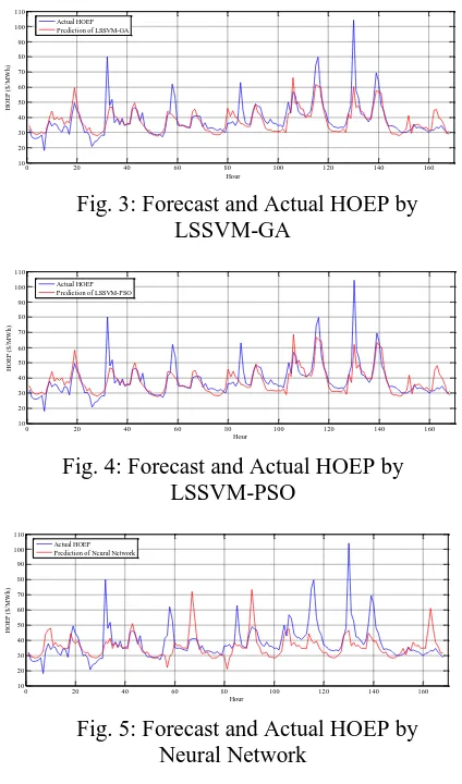
Fig. 3: Forecast and Actual HOEP by LSSVM-GA
Fig. 4: Forecast and Actual HOEP by LSSVM-PSO
Fig. 5: Forecast and Actual HOEP by Neural Network
Figure 2-5 show plots of forecast versus actual HOEP for all models. The first day on testing period was a winter day, hence the forecast models were not able to follow the spike closely. Similar situation happened at point 130 or 10 a.m. on Saturday, 30 January 2010 where the actual HOEP was $104.2/MWh, while the average HOEP for this test data was $38.44/MWh. However, Figure 2 and 3 show that LSSVM-GA and LSSVM-PSO could track the actual data better than the other two models. All of the models were developed on a PC with 6GB of RAM memory and Intel Core i5 2.5GHz processor, while the simulation time of about 20 minutes for GA and LSSVM-PSO was reasonable for day-ahead system operation and decision making.
Conclusion
A hybrid LSSVM and GA for day-ahead electricity price forecasting in Ontario has been
proposed and evaluated. The performance of LSSVM-GA model was compared with those of LSSVM, LSSVM-PSO, NN and another published approaches by a recent research, which apply the same training and testing data [38]. The performance measure was accessed through weekly MAPE, MAE and regression (R). Ontario was found as among the most volatiles power market in the world [51] nonetheless, our hybrid model has shown that the forecast accuracy is also acceptable and better than that obtained by single LSSVM and NN, or other techniques [38]. However, the accuracy on spike areas is quiet low; thus, this issue can be focused on in the future research, research while considering other influential factors such as spot market price and spinning reserve market price [2].
Acknowledgments
We would like to dedicate our appreciation to Universiti Teknikal Malaysia Melaka (UTeM) and National Energy University (UNITEN) for providing financial and moral support throughout conducting this study.
References
[1] D. Niu, D. Liu, and D. D. Wu, “A soft computing system for day-ahead electricity price forecasting,” Appl. Soft Comput., vol. 10, no. 3, pp. 868–875, Jun. 2010.
[2] X. Yan and N. a. Chowdhury, “Mid-term electricity market clearing price forecasting: A hybrid LSSVM and ARMAX approach,” Int. J.
Electr. Power Energy Syst., vol. 53, pp. 20–26,
Dec. 2013.
[3] J. Zhang, J. Han, R. Wang, and G. Hou, “Day -ahead electricity price forecasting based on rolling time series and least square-support vector machine model,” in 2011 Chinese Control and
Decision Conference (CCDC), 2011, pp. 1065–
1070.
[4] W. E. I. Sun, J. Lu, and M. Meng, “Application Of Time Series Based SVM Model On Next-Day Electricity Price Forecasting Under Deregulated Power Market,” P roc. Fifth Int. Conf. Mach.
Learn. Cybern., 2006.
[5] F. J. Nogales, J. Contreras, A. J. Conejo, and S. Member, “Forecasting Next-Day Electricity Prices by Time Series Models,” vol. 17, no. 2, pp. 342– 348, 2002.
Appl. Energy, vol. 77, no. 1, pp. 87–106, Jan. 2004.
[7] P. Mandal, T. Senjyu, N. Urasaki, and T. Funabashi, “A neural network based several-hour-ahead electric load forecasting using similar days approach,” Int. J. Electr. Power Energy Syst., vol. 28, no. 6, pp. 367–373, Jul. 2006.
[8] S. K. Aggarwal, L. M. Saini, and A. Kumar, “Electricity Price Forecasting in Ontario Electricity Market Using Wavelet Transform in Artificial Neural Network Based Model,” Int. J.
Control. Autom. Syst., vol. 6, no. 5, pp. 639–650,
2008.
[9] H. Yamin, S. Shahidehpour, and Z. Li, “Adaptive short-term electricity price forecasting using artificial neural networks in the restructured power markets,” Int. J. Electr. Power Energy Syst., vol. 26, no. 8, pp. 571–581, Oct. 2004.
[10]M. Tsai and C. Chen, “A forecasting system of electric price using the refined Back propagation Neural Network,” 2010 Int. Conf. Power Syst.
Technol., pp. 1–6, Oct. 2010.
[11]V. Vahidinasab, S. Jadid, and a. Kazemi, “Day -ahead price forecasting in restructured power systems using artificial neural networks,” Electr.
Power Syst. Res., vol. 78, no. 8, pp. 1332–1342,
Aug. 2008.
[12]D. Singhal and K. S. Swarup, “Electricity price forecasting using artificial neural networks,” Int.
J. Electr. Power Energy Syst., vol. 33, no. 3, pp.
550–555, Mar. 2011.
[13]P. Areekul, T. Senjyu, N. Urasaki, and A. Yona, “Neural-wavelet Approach for Short Term Price Forecasting in Deregulated Power Market,” J. Int.
Counc. Electr. Eng., vol. 1, no. 3, pp. 331–338,
Jul. 2011.
[14]E. N. Chogumaira, “Short-Term Electricity Price Forecasting Using a Combination of Neural Networks and Fuzzy Inference,” Energy Power Eng., vol. 03, no. 01, pp. 9–16, 2011.
[15]J. P. S. Catalão, S. J. P. S. Mariano, V. M. F. Mendes, and L. a. F. M. Ferreira, “Short-term electricity prices forecasting in a competitive market: A neural network approach,” Electr.
Power Syst. Res., vol. 77, no. 10, pp. 1297–1304,
Aug. 2007.
[16]H. S. Hippert, C. E. Pedreira, and R. C. Souza, “Neural networks for short-term load forecasting: a review and evaluation,” IEEE Trans. Power
Syst., vol. 16, no. 1, pp. 44–55, 2001.
[17]I. A. W. A.R, T. K. Rahman, Z. Z, and A. Ahmad, “Short Term Electricity Price Forecasting Using Neural Network,” in P roceedings of the 4th International Conference on Computing and
Informatics, ICOCI 2013, 2013, no. 042, pp. 103–
108.
[18]T. Niimura and K. Ozawa, “A day-ahead electricity price prediction based on a fuzzy-neuro autoregressive model in a deregulated electricity market,” P roc. 2002 Int. Jt. Conf. Neural
Networks. IJCNN’02 (Cat. No.02CH37290), no. December 1999, pp. 1362–1366, 2000.
[19]P. B. Luh, “Selecting input factors for clusters of gaussian radial basis function networks to improve market clearing price prediction,” IEEE Trans.
Power Syst., vol. 18, no. 2, pp. 665–672, May
2003.
[20]P.-F. Pai, K.-P. Lin, C.-S. Lin, and P.-T. Chang, “Time series forecasting by a seasonal support vector regression model,” Expert Syst. Appl., vol. 37, no. 6, pp. 4261–4265, Jun. 2010.
[21]L. Jinying and L. Jinchao, “Next-day electricity price forecasting based on support vector machines and data mining technology,” 2008 27th
Chinese Control Conf., vol. 630, no. 1, pp. 630–
633, Jul. 2008.
[22]R. a. Swief, Y. G. Hegazy, T. S. Abdel-Salam, and M. . Bader, “Support vector machines (SVM) based short term electricity load-price forecasting,” in 2009 IEEE Bucharest PowerTech, 2009, pp. 1–5.
[23]D. C. Sansom, T. Downs, and T. K. Saha, “Support Vector Machine Based Electricity Price Forecasting For Electricity Markets utilising Projected Assessment of System Adequacy Data,”
in The Sixth International Power Engineering
Conference (IPEC2003), 2003, no. November, pp.
27–29.
[24]T. Wang, “Application of SVM based on rough set in electricity prices forecasting,” 2010 2nd
Conf. Environ. Sci. Inf. Appl. Technol., pp. 317–
320, Jul. 2010.
[25]C. Yan-Gao and M. Guangwen, “Electricity Price Forecasting Based on Support Vector Machine Trained by Genetic Algorithm,” 2009 Third Int.
Symp. Intell. Inf. Technol. Appl., pp. 292–295,
2009.
[26]M. J. Mahjoob, M. Abdollahzade, and R. Zarringhalam, “GA based optimized LSSVM forecasting of short term electricity price in competitive power markets,” in 2008 3rd IEEE
Conference on Industrial Electronics and
Applications, 2008, pp. 73–78.
[27]Y. Wang and S. Yu, “Price forecasting by ICA -SVM in the competitive electricity market,” in
2008 3rd IEEE Conference on Industrial
Electronics and Applications, 2008, pp. 314–319.
Information Technology Application, 2008, pp. 85–89.
[29]J. Tian and Y. Lin, “Short-Term Electricity Price Forecasting Based on Rough Sets and Improved SVM,” 2009 Second Int. Work. Knowl. Discov.
Data Min., pp. 68–71, Jan. 2009.
[30]L. M. Saini, S. K. Aggarwal, and a. Kumar, “Parameter optimisation using genetic algorithm for support vector machine-based price-forecasting model in National electricity market,”
IET Gener. Transm. Distrib., vol. 4, no. 1, p. 36,
2010.
[31]D. C. Sansom, T. Downs, and T. K. Saha, “Evaluation of support vector machine based forecasting tool in electricity price forecasting for Australian national electricity market participants,” J. Electr. Electron. Eng. Aust., vol. 22, no. 3, pp. 227–233, 2002.
[32]J. Zhang and Z. Tan, “Day-ahead electricity price forecasting using WT, CLSSVM and EGARCH model,” Int. J. Electr. Power Energy Syst., vol. 45, no. 1, pp. 362–368, Feb. 2013.
[33]N. Amjady and A. Daraeepour, “Design of input vector for day-ahead price forecasting of electricity markets,” Expert Syst. Appl., vol. 36, no. 10, pp. 12281–12294, Dec. 2009.
[34]H. Shayeghi and A. Ghasemi, “Day-ahead electricity prices forecasting by a modified CGSA technique and hybrid WT in LSSVM based scheme,” Energy Convers. Manag., vol. 74, pp. 482–491, 2013.
[35]J. Zhang, Z. Tan, and S. Yang, “Day-ahead electricity price forecasting by a new hybrid method,” Comput. Ind. Eng., vol. 63, no. 3, pp. 695–701, Nov. 2012.
[36]J. H. Zhao, Z. Y. Dong, Z. Xu, and K. P. Wong, “A Statistical Approach for Interval Forecasting of the Electricity Price,” IEEE Trans. Power Syst., vol. 23, no. 2, pp. 267–276, 2008.
[37]S. Fan, C. Mao, and L. Chen, “Next-day electricity-price forecasting using a hybrid network,” Gener. Transm. Distrib. IET, vol. 1, no. 1, pp. 176–182, 2007.
[38]K. B. Shrivastava, N.A. ; Ch, S. ; Panigrahi, “Price forecasting using computational intelligence techniques: A comparative analysis,”
in 2011 International Conference on Energy,
Automation and Signal, 2011, pp. 1–6.
[39]W. Sun and J. Zhang, “Forecasting Day Ahead Spot Electricity Prices Based on GASVM,” 2008
Int. Conf. Internet Comput. Sci. Eng., pp. 73–78,
Jan. 2008.
[40]V. Vapnik, Statistical Learning Theory. new York: Wiley, 1998.
[41] J. Suykens and K. U. Leuven, “Least Squares Support Vector Machines,” 2003.
[42] H. Wang and D. Hu, “Comparison ofSVM and LSSVM for Regression,” in 2005 International Conference on Neural Networks and
Brain, 2005, no. 5, pp. 279–283.
[43]S. Ismail, A. Shabri, and R. Samsudin, “A hybrid model of self-organizing maps (SOM) and least square support vector machine (LSSVM) for time-series forecasting,” Expert Syst. Appl., vol. 38, no. 8, pp. 10574–10578, Aug. 2011.
[44]D. Çalişir and E. Dogantekin, “A new intelligent hepatitis diagnosis system: PCA–LSSVM,” Expert
Syst. Appl., vol. 38, no. 8, pp. 10705–10708, Aug.
2011.
[45]S. Li and L. Dai, “Classification of gasoline brand and origin by Raman spectroscopy and a novel R-weighted LSSVM algorithm,” Fuel, vol. 96, pp. 146–152, Jun. 2012.
[46]X. Yan and N. A. Chowdhury, “A comparison between SVM and LSSVM in mid-term electricity market clearing price forecasting,” in 2013 26th IEEE Canadian Conference on Electrical and
Computer Engineering (CCECE), 2013, pp. 1–4.
[47]T. Weise, “Global Optimization Algorithms – Theory and Application –,” 2009.
[48]A. Mattiussia, M. Rosanob, and P. Simeoni, “A decision support system for sustainable energy supply combining objective and multi-attribute analysis: An Australian case study,”
Decis. Support Syst., vol. 57, pp. 150–159, 2014.
[49]P. Kaur and J. Kaur, “Fingerprint Recognition Using Genetic Algorithm and Neural Network,”
Int. J. Comput. Eng. Res., vol. 3, no. 11, pp. 41–
46, 2013.
[50]Q. Bai, “Analysis of Particle Swarm Optimization Algorithm,” Comput. Inf. Sci., vol. 3, no. 1, pp. 180–184, 1998.