Data Selection and Fuzzy-Rules Generation for Short-Term Load Forecasting Using ANFIS

DOI: _{10.12928/TELKOMNIKA.v14i3.3413}  ₇₉₁

Data Selection and Fuzzy-Rules Generation for

Short-Term Load Forecasting Using ANFIS

M. Mustapha, M. W. Mustafa*, S. N. Khalid

Faculty of Electrical engineering, universiti Teknologi Malaysia, 81310, Johor, Johor bahru, Malaysia *Corresponding author, e-mail: wazir@fke.utm.my

Abstract

This paper focused on data analysis, with aim of determining the actual variables that affect the load consumption in short term electric load forecasting. Correlation analysis was used to determine how the load consumption is related to the forecasting variables (model inputs), and hypothesis test was used to justify the correlation coefficient of each variable. Three different models based on data selection criteria where tested using Adaptive Neuro-Fuzzy Inference System (ANFIS). Subtractive Clustering (SC) and Fuzzy c-means (FCM) rules generation algorithms ware compared in all the three models. It was observed that forecasting using Hypothesis test data with SC algorithm gave better accuracy compared to the other two approaches. But FCM algorithm is faster in all the three approaches. In conclusion, hypothesis test on the correlation coefficient of the data is a commendable practice for data selection and analysis in short-term load forecasting.

Keywords: short-term load forecasting, anfis, clustering algorithm, correlation analysis, hypothesis test

Copyright © 2016 Universitas Ahmad Dahlan. All rights reserved.

1. Introduction

Factors influencing energy consumption plays a vital role in its determination. They are the key parameters used to forecast electricity load consumption. Depending on the forecasting horizon, these parameters vary from weather variables, economic variables, customer class and demographic or population factors. Some research works restrict on two or more variables, and others used only historical load data. For example, variation in the load consumption corresponds to time of the day, week, month or temperature of forecasting area and behaviour of customers towards electricity usage [1].

The first stage in obtaining accurate load forecasting is proper data processing. This gives the reason why power system organization are gathering the relevant data because of its significant influence in their business activities [2]. Such information received from data processing and analysis give a clue on which method to be used or how to use it. It is also easy to determine when the consumption is low or high in the load profile, or the relationship between the consumption and these variables. Even though, it is difficult to determine the exact relation between the load consumption and forecasting variables. Because, different variables affect the load in different way. The degree of the effect may be high or low, or even negative [3]. As suggested in [4], the factors being reduced, there by making the model simple and easy to use, and subsequently give room for determining the actual parameters that influence the load consumption.

define exact variables that will affect the load consumption. Correlation analysis and hypothesis test are used to determine exact variables that influence the load consumption.

This paper addresses the issue of reducing the number variables through correlation analysis and hypothesis test. It also applied SC and FCM to minimize the number of rules and slowness of the model due to high value of predictors.

2. Model Development

In this work, ANFIS will be used to map the forecasting variables (model inputs) to corresponding load consumption (model output). It is aimed at generating a model that will not only be familiar with the training set, but also be able to map the test inputs to the test outputs. To achieve this it is necessary to determine the variables that influence the load consumption, and model functions that will give a good and accurate mapping between these variables. In this work test of hypothesis on correlated data is used to select the input variables. Correlation analysis and test of hypothesis are discussed in the section below.

2.1. Correlation Analysis and Hypothesis Test

Correlation is the measure of interrelation between the changes in two variables. It estimates how changes in one variable affect another. It describes the relation between two pairs of data. Correlation coefficient (R) ranges from -1 to +1. Any value within this range determines the relationship between the variables [9]. High value (close to +1 or -1) indicates strong relationship and value close to zero indicates low correlation. Zero correlation coefficient shows that there is no any relation between the two pair of the data. In other words knowing x cannot assist in determining y. Correlation coefficient R, between two set of data can be calculated using the following formula:

 

cov

,

xy

x y

x y

R

 



(1)

Where

cov



x y

,



is the population covariance,



_xand



_y are the population individual

standard deviation. If the input vector is X [Xr1 Xr2 Xr3 ………Xrc], the corresponding output

vector is Yr. Where r donates rows and c donates columns. The output has only one column

with a number of rows. Correlation analysis is carried out using equation (1) between any element of Xrc (x) and corresponding element of Yr (y). Thus results in c-number of correlation

coefficients.

Hypothesis test is a method used at the data analysis stage of comparative analysis between a set of experimental data. The purpose is to determine the significance of an empirical analysis using p-value. This is the smallest level of significance that will lead to acceptance or rejection of the null hypothesis. It is the area shaded around the two tail ends of normal distribution curve. The first step is by setting a null hypothesis and alternative hypothesis on the observation, followed by pre-setting an α-value. Then compute the p-values and deduce conclusion. From [9], p-value is computed using the relation:

(2)

Where Zi is the Z-value corresponding to one side of the hypothesis and Zj is the Z-value

corresponds to the other side.

For two-sided hypothesis (Zi and Zj).

1 (3)

2.2. Adaptive Neuro Fuzzy Inference System (ANFIS)

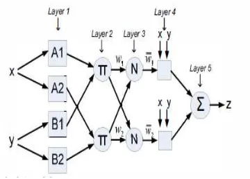
ANFIS (developed by J. S. Roger in 1993) combines the advantages of fuzzy systems and neural-networks [10]. Is a network-based structure (figure 2) that uses the Sugeno-type ‘IF…..THEN’ rules and Neural Network (NN). It uses hybrid learning in which the consequent parameters are determined by Least Square Algorithm (LSA) in the forward pass. In the backward pass error measures are disseminated backward through every node, and the premise parameters (parameters associated with the membership function) are updated using Gradient Decent Algorithm (GDA). Figure 2 shows a typical ANFIS structure with only two inputs (x and y) and one output (z). The structure consists of five layers with several nodes (depending on the number of input variables and linguistic variables). For a data point xi, ANFIS computes a corresponding output yi.

For a first order Sugeno-type fuzzy system with only two inputs, the rules are: 1. If x is A1 and y is B1, then

f

₁



p x

₁



q y

₁



r

₁

2. If x is A2 and y is B2, then

f

₂



p x q y

₂



₂



r

₂

Where

p

_i,

q

_i and

r

_i are the consequent parameters.

0 10 20 30 40 50 60 70 80 90 100 110 120 130 140 150 160 170 180 800

900 1000 1100 1200 1300 1400

H

our

ly

Lo

ad

C

o

ns

u

m

pt

ion (

M

W

)

Time (hrs)

Hourly Load Consumption

Figure 1. Hourly load pattern for seven days (5th to 11th May, 2014)

Figure 2. Typical ANFIS structure

If

o

_ijis the output of node i in layer j, the function of each node can be explained from node to node on layer basis:

Layer 1: Each node in this layer is an adaptive node, whose output is determined by the membership function (MF) in that node. The MF fuzzify the input variable xi in that node. For

node A1 the output is given by:

 

1

i

A

i

µ

i

o



x

(4)

Where x is an input to node ‘i’ and Ai is linguistic level associated with this node

i

A

µ

is the

membership function (MF) of A. generally,

o

_ijis the membership grad of a fuzzy set A which can be any MF such as the guassian MF of Equation (5):

 

2

1 2

i i i

x c

A i

µ

x

e



       



(5)

Layer 2:Every node of this layer is a fixed node. Its output is the firing strength of all the signals entering the node from the previous layer. Thus:

2

...

i i Ai Bi Ci

o

_



w



µ



µ



µ

(6)

Layer 3: This is normalization layer. The output of each node here is the ratio of the node’s fairing strength to the sum of all the firing strengths of the other nodes, thus:

3

1 2

...

i

i i

w

o

w

w

w









(7)

Layer 4: Output of each node in this layer is:

4

(

)

i i

i i i i i

o



w f



w p x q y r





(8)

Layer 5: In this layer, the only output node will sum up all the output signals of layer 4, thus:

5

i

i i

i

o





w f

(9)

This gives the overall output, z.

2.3. Fuzzy Rules Generation

A Sugeno-type, “IF…THEN” Fuzzy rules is a parameter identification problem which require membership function tuning. Among the methods presented to determine the fuzzy rules we will focus on FCM and subtracting clustering. Fuzzy clustering is used to classify data in to different groups based on number of clusters. A data sample can be in a number of cluster groups which are identified by their degree of membership [11]. This will reduce the computational burden on the system.

2.3.1. SC Method

This is a method developed by Chiu to identify fuzzy models [12]. This method is introduced to identify, naturally, a group of data that will represent the general behaviour of the system. It is aimed at reducing the computational burden in large data systems. Depending on the nature of the problem, the algorithm involves computing density measure of every data point. Thus, for every data point xi, the density measure is given by:

2

2 1

exp

(

2)

n

i j

i

j a

x

x

D

r



























(10)

Where ra is the radius that determines the neighbourhood around the data centre, and n is the number of data points. According to [12]

0.15

 

r

a

0.3

, therefore 0.2 is choosen in this work.

For all the three cases initial cluster is selected based on the data point with the highest density. Now if xc1 is that cluster centre with the density measure Dc1, then the next density

measure for another data point xi can be deduced from the relation.

2 1 1

exp

2

(

2)

i c

i i c

b

x

x

D

D

D

r











 











(11)

We make rb greater than ra to disperse the clusters. Typically rb = 1.5ra [12]. Same procedure is

followed to determine other cluster centres until a sufficient number is reached.

2.3.2. Fuzzy C-Means Clustering (FCM)

Like the SC, FCM [13] is used to reduce the model complexity through reduction in the number of membership functions. FCM uses fuzzy partitioning in which a particular data point belongs to a number of clusters with different degree of membership. The algorithm is based on optimization of basic c-means objective function of equation (12):





 

2

1 1

,

c n

m

m ik j i

i j

J

U C



c

x

 







(12)

Subject to:

1

1

c

ij i









,

1

 

i

n

, 1

 

j

c

n

is the number of data vectors and

c

is the number of clusters,

m



1

is used to adjust the weights associated with membership function.

U

is the fuzzy partition matrix which contains the membership of each feature vector for each cluster. The cluster matrix is given by:



1, 2, ,...,3 c



,

C c c c c

(13)

Where

c

_iis a cluster centre of the fuzzy group and can be computed using:

 

 

1 1

;

n _m n _m

i ij j ij

j j

c



x



 







1

 

i

c

(14)



can be obtain using the following equation:





2 1

1

1

,

/

ji c

m

ij jk

k

d

d



 





for

d

ij

 

c

i

x

j (15)

FCM is an iterative algorithm which involves few to compute the cluster centres and member ship functions.

Step 1: We initialized the membership matrix randomly within the interval [0,1] Step 2: Equation (14) is used to compute the cluster centres.

Step 3: Equation (12) is used in computing the cost function and final value was obtained after there is no significant change in the iteration.

Step 4: Using the cluster centres new



_jiis computed.

Step 5: Repeat steps 2 to 4.

Both the algorithms determined the cluster centres and subsequently the membership matrix. This reduced the number of membership functions and therefore speeds the algorithm with the required accuracy.

3. Short-Term Load Forecasting Implementation

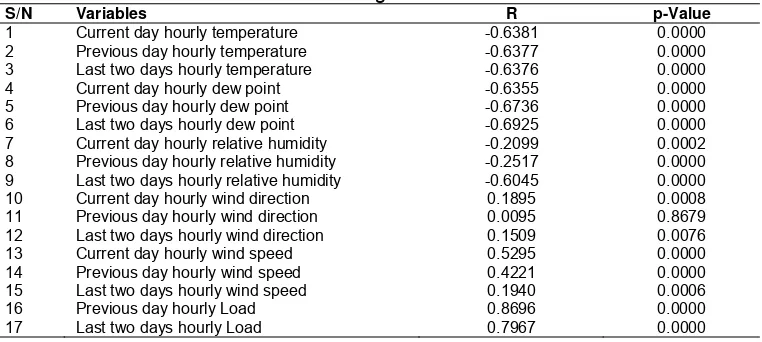
load consumption. Out of the four season, data collected in the spring is considered for this work. Spring starts from middle of March to the Middle of June. Data of three days (Tuesday, Wednesday and Thursday) in each week, from 18th of March to 10th of June 2014 is used. First nine weeks for training and last four weeks for testing. Meaning that two months data for training and first week of next month for testing. The data is classified base on the correlation analysis and hypothesis test. The first class of data comprised all the available data collected from the utility company and the weather station. This covers load consumption, temperature, dew point, relative humidity, wind speed and wind direction. Second class comprised of data extracted from the first class. It is built based on the correlation analysis. Correlation coefficient is computed for every variable, any one with value less than 0.5 are rejected from the list. The last set is that of the data based on the test of hypothesis results on the correlation coefficient. Fixed significance value test is used in testing the significance of the correlation on the data. All data with p-value less than the α-value are also rejected. The data used is presented in table 1. Because the the load consumption is similar throughout the week days, Tuesday, Wednesday and Thursday data is considered the forecasting.

3.1. Correlation Coefficient and Test of Hypothesis

Generally, determining the actual variables using correlation analysis and hypothesis test to validate the correlation is a good practice. In this study, we used correlation analysis to determine the relationship between the load consumption and the load forecasting variables. Hypothesis test is used to justify the correlation coefficients of every variable against the load. Following computing the correlation coefficientR, between the load consumption and the forecasting variable, we then define the null hypothesis H₀and the alternative hypothesisH₁. Now let:

H0 = the correlation between the load consumption and the forecasting variable is by

random chance

H1 = the correlation between the load consumption and the forecasting variable is not

by random chance.

For this purpose, Z-test will is used to determine the P-value of each forecasting variable using equation (2). Now we set the α-value to a fixed significance value of 0.0005. If the computed P-value is greater than this value the null hypothesis will be rejected. And subsequently reject the variable in the forecasting. Table 1 shows the computed

R

and P-values and the deduced conclusion based on the P-value.

From the tested variables some are rejected based on the correlation coefficient, because their correlation coefficient is less than ±4.000. For the hypothesis test, some variables are also rejected because their P-values are more than the fixed significance value (α-value). Therefore their correlation is by random chance.

Table 1. Correlation Coefficients (R) and Hypothesis Test (p-values) for Training and Testing Data

S/N Variables R p-Value

1 Current day hourly temperature -0.6381 0.0000

2 Previous day hourly temperature -0.6377 0.0000

3 Last two days hourly temperature -0.6376 0.0000

4 Current day hourly dew point -0.6355 0.0000

5 Previous day hourly dew point -0.6736 0.0000

6 Last two days hourly dew point -0.6925 0.0000

7 Current day hourly relative humidity -0.2099 0.0002

8 Previous day hourly relative humidity -0.2517 0.0000 9 Last two days hourly relative humidity -0.6045 0.0000

10 Current day hourly wind direction 0.1895 0.0008

11 Previous day hourly wind direction 0.0095 0.8679

12 Last two days hourly wind direction 0.1509 0.0076

13 Current day hourly wind speed 0.5295 0.0000

14 Previous day hourly wind speed 0.4221 0.0000

15 Last two days hourly wind speed 0.1940 0.0006

16 Previous day hourly Load 0.8696 0.0000

3.2. Load Forecasting Using the Developed Model

As stated in section 5, three sets of data obtained from the correlation analysis and the test of hypothesis are used. Case 1: in which all the data sets will be used without the correlation analysis and hypothesis test. This generates a 216 by 18 data points. Case 2: in which variables with correlation coefficients greater than ±4 are considered, thus, 11 variables are selected from that of case 1. Case 3: in which the variables with significance level above 0.0005 are considered. Thus, 14 variables are selected from that of case 1. ANFIS is applied to forecast the load using the data of these three Cases, in order to compare their accuracy. Also, SC and FCM will be used to generate the fuzzy rules.

ANFIS was used to forecast the load using these three case scenarios. It is chosen because it has the advantage of enduring the uncertainties in a large noisy data, and it is good in pattern learning and computationally effective [14, 15]. To simplify the mathematical difficulties, two techniques for number of fuzzy rules reduction are considered. The first model is using FCM and the second is using SC. Not only the accuracy, these methods also, improved the forecasting time. For both the two methods and the three cases the results obtained are described in section 4.

The three experiments (cases) ware carried out in windows 8.1, 64 bit Operating System computer, with core i5 @ 1.70GHZ speed and 8GB RAM. The results obtained are below, and in Table 2.

Figure 3. Plot of actual and forecasted load using SC for all data

Figure 4. Plot of actual and forecasted load using FCM for all data

10 20 30 40 50 60 70 80 90 100 800 900 1000 1100 1200 1300

1400 _{Actual Load}

Forecasted Load Time (hrs) A c tual Load (M W ) 800 900 1000 1100 1200 1300 1400 For e cas ted Loa d ( M W )

Figure 5. Plot of actual and forecasted load using SC for correlation data

Figure 6. Plot of actual and forecasted load using FCM for correlation data

4. Results Discussion

For all the three cases Mean Square Error (MSE), Root Means Square Error (RMSE) and Mean Absolute Percentage Error (MAPE) are used to evaluate the accuracy of the experiment.

 

10 20 30 40 50 60 70 80 90 100 800 900 1000 1100 1200 1300 1400 Actual Load Forecasted Load Time (hrs) A c tual Load ( M W ) 800 900 1000 1100 1200 1300 1400 For e cast ed Load ( M W )

10 20 30 40 50 60 70 80 90 100 800 900 1000 1100 1200 1300 1400 Actual Load Forecasted Load

Time (hrs) (hrs)

A c tual L oad ( M W ) 800 900 1000 1100 1200 1300 1400 F or ecas ted Loa d ( M W )

10 20 30 40 50 60 70 80 90 100 800 900 1000 1100 1200 1300 1400 Actual Load Forecasted Load

Time (hrs) (hrs)

Case 1: Here all data sets as presented in Table 1 are used. Figure 3 shows the graph5 of actual load and predicted load for SC and Figure 4 for FCM. An MSE of 1785.95, RMSE of 42.26 and MAPE of 3.30% are obtained. For Fuzzy c-means algorithm Figures 5 and 6 respectively, show the plot of actual and forecasted load and forecasting error with MSE of 1734.40, RMSE of 41.65 and MAPE of 3.45%.

Case 2: Here the data is selected based on the results of the correlation coefficients. Out of the 17 tested variables, 6 are rejected because their correlation coefficients are less than ±4.000 (refer to Table 1). Figure 5 shows the plot of actual load and predicted load for SC and Figure 6 for FCM. For SC MSE of 1140.13, RMSE of 33.77 and MAPE of 3.01% are obtained. For FCM algorithm an MSE of 1328.95, RMSE of 36.45 and MAPE of 3.15% were obtained.

Casa 3: The data used in this Case is selected based on the results of the correlation coefficients and hypothesis test (refer to Table 1). Figure 7 shows the plot of actual load and predicted load for SC and Figure 8 for FCM. An MSE of 613.89, RMSE of 24.78 and MAPE of 2.19% are obtained for SC. For the FCM an MSE of 816.34, RMSE of 28.57 and MAPE of 2.23% were obtained.

Also, Table 2 shows the number of rules generated and the speed of corgence in each case. For SC algorithm, case 1 produce highest number of rules, and case 2 produce lowest. For FCM the number of rules are same and lower than that of SC in all the cases. Also highest speed is recorded in case 1using SC and FCM recorded the lowest speed in all the case.

0 20 40 60 80 100

800 900 1000 1100 1200 1300 1400

Actual Load Forecasted Load

Time (hrs)

Act

ua

l Lo

ad (

M

W

)

800 900 1000 1100 1200 1300 1400

Fo

rec

as

te

d Loa

d (

M

W

)

0 20 40 60 80 100

800 900 1000 1100 1200

1300 Actuald Load Forecasted Load

Time (hrs)

A

c

tu

al

d Loa

d (

M

W

)

800 900 1000 1100 1200 1300

Fo

re

c

a

s

te

d

Loa

d (

M

W

)

Figure 7. Plot of actual and forecasted Load using SC for hypothesis data

Figure 8. Plot of actual and forecasted Load using FCM for hypothesis data

Table 2. Performance evaluation and comparison of the three cases

Data used Fuzzy rules generation

method

Number of Fuzzy rules generated

Error measurement Computation time (sec)

MSE RMSE MAPE (%)

Case 1 FCM 15 1734.40 41.65 3.45 27.65

SC 184 1785.95 42.26 3.30 12258.83

Case 2 FCM 15 1328.95 36.45 3.15 22.03

SC 68 1140.13 33.77 3.01 472.30

Case 3 FCM 15 816.34 28.57 2.23 29.56

SC 107 613.89 24.78 2.19 2195.33

5. Conclusion

Acknowledgements

The authors acknowledge Malaysian Ministry of higher Education and Universiti Teknologi Malaysia for supporting this work.

References

[1] A Jain, B Satish. Clustering based Short Term Load Forecasting using Support Vector Machines. In

Proceeding of 2009 IEEE Bucahrest Power Tech. 2009: 1-8.

[2] A Chakravorty, C Rong, P Evensen, T Wlodarczyk, Wiktor. A Distributed Gaussian-Means Clustering

Algorithm for Forecasting Domestic Energy Usage. International Conference on Smart Computing.

2014: 229-236.

[3] S Mirasgedis, Y Sarafidis, E Georgopoulou, DP Lalas, M Moschovits, F Karagiannis, D

Papakonstantinou. Models for mid-term electricity demand forecasting incorporating weather

influences. ENERGY. 2006; 31: 208-227.

[4] J Zhu. The Optimization Selection of Correlative Factors for Long-term power load Forecasting. IEEE

Fifth Int. Conf. Intell. Human-Machine Syst. Cybern. 2013: 241–244.

[5] Y Chen, PB Luh, C Guan, Y Zhao, LD Michel, MA Coolbeth, PB Friedland, SJ Rourke, S Member.

Short-Term Load Forecasting : Similar Day-Based Wavelet Neural Networks. IEEE Trans. Power

Syst. 2010; 25(1): 322–330.

[6] N Sovann, P Nallagownden, Z Baharudin. A method to determine the input variable for the neural

network model of the electrical system. 2014 5th Int. Conf. Intell. Adv. Syst. 2014: 1-6.

[7] H Quan, D Srinivasan, A Khosravi. Short-Term Load and Wind Power Forecasting Using Neural

Network-Based Prediction Intervals. IEEE Trans. Neural Networks Learn. Syst. 2014; 25(2): 303-315.

[8] FL Quilumba, W Lee, H Huang, DY Wang, S Member, RL Szabados. Using Smart Meter Data to Improve the Accuracy of Intraday Load Forecasting Considering Customer Behavior Similarities.

IEEE Trans. Smart Grid. 2015; 6(2): 911-918.

[9] DC Montgomery, GC Runger. Applied Statistics and Probability for Engineers. Third Edition. USA: WILEY. 2002.

[10] JR Jang. ANFIS: Adaptive-Network-Based Fuzzy Inference System. IEEE Trans. Syst. Man Cybern.

1993; 23(3): 665-685.

[11] Z Feng, B Zhang. Fuzzy Clustering Image Segmentation Based on Particle Swarm Optimization.

TELKOMNIKA Telecommunication Computing Electronics and Control. 2015; 13(1): 128-136.

[12] SL Chiu. Fuzzy Model Identification Based on Cluster Estimation. J. Intell. Fuzzy Syst. 1994; 2:

267-278.

[13] JC Bezdek, R Ehrlich, W Full. FCM : The Fuzzy C-Means Clustering Algorithm. Comput. Geosci.

1984; 10(2): 191-203.

[14] A Azriyenni, MW Mustafa. Application of ANFIS for Distance Relay Protection in Transmission Line.

Int. J. Electr. Comput. Eng. 2015; 5(6).

[15] PK Pandey, Z Husain, RK Jarial. ANFIS Based Approach to Estimate Remnant Life of Power