Modelling Of Non-Reverberant Acoustic Space Using Statistical Energy Analysis (Sea).

(1)

MODELLING OF NON- REVERBERANT ACOUSTIC SPACE USING STATISTICAL ENERGY ANALYSIS (SEA)

GOH JZUN HWEE

This report is submitted in partial fulfillment of requirements for the award of Bachelor Degree of Mechanical Engineering (Automotive)

Faculty of Mechanical Engineering Universiti Teknikal Malaysia Melaka

(2)

ii

SUPERVISOR DECLARATION

“I hereby declare that I have read this thesis and in my opinion this report is sufficient in terms of scope and quality for the award of the degree of

Bachelor of Mechanical Engineering (Automotive)”

Signature: ………..

Supervisor: ………..

(3)

iii

DECLARATION

“I hereby declare that the work in this report is my own except for summaries and quotations which have been duly acknowledged.”

Signature: ……….

Author: ……….

(4)

iv

DEDICATION

To My Beloved Family

Goh Hock Lim

Tan Siew Wah

Goh Yau Li

Goh Li Nee

(5)

v

ACKNOWLEDGEMENTS

Firstly, I would like to express my greatest gratitude to my supervisor Dr. Azma Putra. From his guidance and support, I am able to accomplish this research in the period given.

Besides, I sincerely thank to those who are directly or indirectly involve in making this report. Thank to master student Al Munawir who taught me how to conduct the experiment and progress the result of this research (PSM). Special thanks to Mr. Junaidi, Mr. Alizam, Mrs. Nur Hidayah and Mr. Hasrul Hadi for teaching and guide me in using lab equipments. Besides, I would like to thank to my panel for the presentation, Dr. Roszaidi, Mr. Hamzah and Dr. Musthafah for giving me a good critic and suggestion.

(6)

vi

ABSTRAK

(7)

vii

ABSTRACT

(8)

viii

3.1 The Classical Sea Model 10

(9)

ix

CHAPTER CONTENTS PAGE

3.2 Corrected Sea Model 13

CHAPTER 4 EXPERIMENTAL WORK 15

4.1 Measurement 15

4.1.1 Reverberant Condition 16

4.1.2 Non-Reverberant Condition 18

4.2 Signal Post-Processing 19

CHAPTER 5 RESULT AND ANALYSIS 21

5.1 Result 21

5.1.1 Reverberant Condition 21

5.1.2 Non-Reverberant Condition 23

CHAPTER 6 CONCLUSION AND RECOMMENDATION 30

6.1 Conclusion 30

6.2 Recommendation 30

REFERENCES 31

(10)

x

LIST OF TABLES

NO TITLE PAGE

4.1 List Of Equipment Used In The Coupled Boxes Experiment

(Reverberant Condition) 17

4.2 List Of Equipment Used In The Coupled Boxes With Added

(11)

xi

LIST OF FIGURES

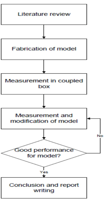
1.1 Methodology Flow Chart 4

1.2 Coupled Box 5

1.3 Cad Drawing Of Coupled Box 6

2.1 The Reverberant Field; Illustration Of The Reflections In An Enclosed Space Compared To Direct Sound At A Variable

Distance From The Sound Source(Rayburn, 2011). 7 2.2 Block Diagram Of The Sea Model With Pin The Input Power

To Subsystem 2 (Vestibule 1), Pi,J The Power Transfer

Between Subsystems And Pid The Losses (Forssén, Et Al.). 9

3.1 A Schematic Diagram Of Sea Model 10

4.1 Diagram Of The Coupled Boxes Experiment Measurement

Setup (Reverberant Condition). 16

4.2 Diagram Of Subsystems With Added Trim Sponges

Experiment (Non-Reverberant Condition). 18

4.3 Measured Sound Absorption Coefficient Of The Sponge

Material Using In The Experiment. 18

4.4 Diagram Of Methodology To Remove Direct Field

Component. 19

5.1 Measured Normalized Energy In The Subsystems With

Power Injected In Subsystem 1. 21

5.2 Measured Normalized Energy In Subsystems With Power

(12)

xii

5.3 Coupling Loss Factor From Experimental Sea In A

Reverberant Condition. 22

Injected In Subsystem 1. 23

Injected In Subsystem 2. 23

5.6 Impulse Response Of Subsystem 1 With Power Injected In Subsystem 1 Before And After Removal Of Direct Field

Components. 24

5.7 Measured Normalized Energy Of Subsystem 1 With Power Injected In Subsystem 1 Before (-) And After(- -) Removal

Of The Direct Field Components. 24

Components. 25

5.9 Measured Normalized Energy Of Subsystem 1 With Power Injected In Subsystem 2 Before (-) And After (- -) Removal

5.10 Impulse Response Of Subsystem 2 With Power Injected Subsystem 1 Before And After Removal Of Direct Field

Components. 26

(13)

xiii

5.14 Coupling Loss Factor From Experimental Sea In A Non-Reverberant Condition Before Removal Of Direct Field

Components. 28

5.15 Coupling Loss Factor From Experimental Sea In A Non-Reverberant Condition After Removal Of Direct Field

(14)

xiv

NOMENCLATURES

i

 = Mean Absorption Coefficient Of The Surface

c = Speed Of Sound, ms-1

L = Matrix Of Coupling And Damping Loss Factors

Mo = Modal Overlap Factor

N = Total Number

N2 = Large Dimension Of Energy Matrix

Nm = Modal Number

Pi,j = Power Transfer Between Subsystems Pid = Power Losses Between Subsystems

i

S = Surface Area Of Partition Between Subsystems

x x

S = Auto-Spectra From The Reference Microphone

y y

(15)

xv

NOMENCLATURES

y x

S = Cross-Spectra Between The Two Microphones

ij

 = Transmission Coefficient

a

t = Arrival Time Of The First Reflection, s

V = Volume, m3



₌ Centre Frequency Of Band B Or Radian Frequency, rad/s

 

t

(16)

xvi

LIST OF APPENDICES

NO. TITLE PAGE

A Gantt Chart For PSM 1 35

B Gantt Chart For PSM 2 36

C Hand Grinder BOSCH 37

D Silicone Araldite 37

E Trim Sponge 38

F LDS Dactron Photon+ Signal Analyzer 38

G 5 Watt Loudspeaker 39

H Dimension Of The Room 39

I Measurement Noise Of Coupled Boxes (Reverberant

Condition) 40

J Measurement Noise Of Coupled Boxes With Added Trim

Sponges (Non-Reverberant Condition) 40

K Partition With An Opening 41

(17)

1

CHAPTER 1

INTRODUCTION

1.1 BACKGROUND

Early, 1990s, image source and ray tracing methods were commonly used to solve the calculation of interior noise at higher frequencies. More recently, Statistical Energy Analysis (SEA) methods have been commonly used to solve this problem (David, 2009). The development of SEA is in 1960 by Richard Lyon to investigate random vibration and vibration energy flow in structures. The relationship of power and energy was determined. The power flow was proportional to the difference in uncoupled energies of the resonators thus it always flows from the resonator of higher to lower resonator energy. A complex structure is divided into ‟subsystems‟ and then stored and exchanged vibrational energy between these subsystems are analyzed. Several advantages found by the energy-based approach used in SEA such as the energy quantities can be averaged more easily. However, there is a requirement that the subsystem must vibrate in resonant mode where modal overlap is high in a frequency band. In this condition, the details of the response are ignored, but rather the ‟statistical‟ average of the data. In 1960, SEA developed that Smith‟s limiting vibration amounted to an equality of energy between the resonator and the mean modal energy of the sound field. Both calculations were therefore consistent and power flow between resonators until equilibrium (Lyon & DeJong, 1995).

(18)

2

important to predict the energy distribution. Prediction of system damping has improved. Although the improvements were not particularly related to SEA experiment, the experiment by Heckl (1962) on plate boundary absorption has found that the way of absorption coefficients vary with frequency is primarily a function of the geometry of the boundary structure. The SEA method of calculating the coupling loss factor between room and cavity given by Price and Crocker (1969) has proven that transmission from room to cavity is similar with transmission from room to room.

In recent years, Ming and Pan (2004) predicted the insertion loss of acoustical enclosures in different frequency ranges. SEA method has been also successful investigated of structural response and noise reduction of an acoustical enclosure by Lei (2012). According to Ahmida and Arruda (2003), the SEA coupling loss factor model has been estimated via the Spectra Element Method (SEM). SEA can be used for prediction of the interior sound field in vehicle (Forssen, 2012), prediction of Sabine absorption coefficient of modally reactive panels (Sum & Kim Seng, 2005), prediction sound transmission through double walls with using coupling loss factor room to cavity undertimes the coupling (Robert, 2003), prediction of impact sound transmission in building acoustic (Kim & Shon, 2001) and prediction of transmission loss in building structures (Koizumi & Tsujiuchi, 1999).

SEA is a method for mid to high frequency noise and vibration analysis. This technique assumes that a component (subsystem) of a structure contains a large number of local modes that cannot be modeled precisely (Belyaev & Langley, 2010). For the case of an acoustic space subsystem, the space should be made up of diffuse or reverberant sound field. According to Sarradj (2004), SEA model can be divided into subsystems and there are no formal criteria and no systematic approach for division. Subsystems are physical element of the structure which there is dissimilar discontinuities in physical properties (thickness, mass density, wave type etc). As excitation is subjected to the subsystem and then turn off, the subsystem should vibrate in resonant mode. That mean the vibration energy stored in the subsystem was decay. Thus, a reverberant sound field exists within the subsystem. Some examples of vibro acoustic subsystems are listed such as an acoustic cavity (a room), a plate, a beam, shells, and non-isotropic plates.

(19)

non-3

resonant response is similar to the conventional SEA modelling for resonant response but uses different expressions for the coupling loss factor. SEA are widely used in aerospace industry, ship building industry and building acoustics, and efforts have been undertaken to model vibration transmission through structural junctions. Meanwhile, SEA started involves in commercial software like the other analysis methods (2010).

1.2 PROBLEM STATEMENT

The treatment of an acoustic space with absorber materials such as the car interior makes it space not fully reverberant, but dominates by the direct field component. Therefore, the classical SEA model might fail to predict the „correct‟ sound pressure level.

1.3 OBJECTIVE

This project consists of the following objectives:

1. To investigate the effect of direct field component on a SEA model of acoustic space subsystems.

2. To investigate the sound field inside an acoustic space using the corrected SEA model by eliminate direct field component.

(20)

4

1.4 METHODOLOGY

Figure 1 1: Methodology flow chart

(21)

5

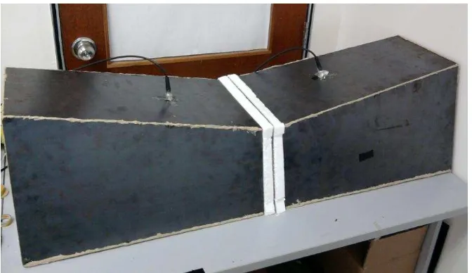
edges of the box for sound insulation. The next step will be the measurement in coupled box. The coupled box can be easily controlled by placing absorbent materials on the room walls to reduce the reverberant effect. Measurement is conducted in the box separated by a solid partition made of same material with an opening of 50 x 50 mm at the middle for reverberant condition and non-reverberant condition. The power injection technique is implemented to obtain the coupling loss factor.

Figure 1.2: Coupled box

(22)

6

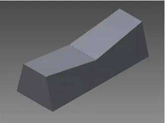
Figure 1.3: Cad drawing of coupled box

Figure 1.3 shows the cad drawing of coupled box by Autodesk Inventor.

1.5 SCOPE

1 The experiment is simulated using two coupled boxes which is easy to control.

(23)

7

CHAPTER 2

LITERATURE REVIEW

Noise can be classified into two categories, namely structure borne and airborne. Structure-borne is noise that produced by direct vibration of the walls. Airborne noise is noise generated through the air before reaching a partition. These noises can be insulated by adding sound dampening materials (Hosseini Fouladi,et.al. 2009).

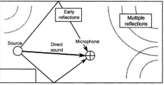
Reverberant field is a free field that exists only under specific test conditions. Outdoor condition can approach it. Indoors, the interaction of the reverberant field and direct field can be observed as the sound source is moved away. Figure 2.1 shows the illustration of the reflections in an enclosed space compared to direct sound at a variable distance from the sound source (Rayburn, 2011).

Figure 2 1: The reverberant field; illustration of the reflections in an enclosed space compared to direct sound at a variable distance from the sound source (Rayburn,

(24)

8

Ribeiro and Smith (2005) investigate sound pressure level distribution due to one or more sound sources in a large acoustic space by using SEA. The sound field inside an industrial workroom may be predicted by the resulting model. It is generally not possible to assume the a uniform reverberant field throughout the room due to the attenuation and scattering of the sound field with distance in such spaces. A separate treatment of direct field and reverberant sound fields was predicted on the model. Application of corrections such as barrier theory was required for the direct sound field which was assumed to be free-field propagation (no obstacles are located between the source and the receiver). SEA framework with the power input corrected for energy lost at first reflection was used and analyzed for the variation of the reverberant field around the room. The sum of the direct field and reverberant fields represent the total sound pressure level at any receiver point. Three distinct subsystems were formed from the acoustic space for measurements of a workroom using experimental SEA methods. The presence of direct field affected the SEA parameters result Experimental and theoretical predicted SEA parameters have been compared. The coupling loss factors shown good agreement but the damping loss factors estimated were less well with the measured data.