Quantifying haze from satellite using Haze Optimized Transformation (HOT).

http://dx.doi.org/10.12988/ams.2015.5130

Quantifying Haze from Satellite Using Haze

Optimized Transformation (HOT)

Muhammad Fahmi Razali, Asmala Ahmad, Othman Mohd, Nurul Iman Saiful Bahari

Centre for Advanced Computing Technology (C-ACT) Faculty of Information and Communication Technology Universiti Teknikal Malaysia Melaka (UTeM), Malaysia

Hamzah Sakidin

Department of Fundamental and Applied Sciences Faculty of Science and Information Technology Universiti Teknologi PETRONAS (UTP), Malaysia

Copyright © 2015 Muhammad Fahmi Razali et al. This is an open access article distributed under the Creative Commons Attribution License, which permits unrestricted use, distribution, and reproduction in any medium, provided the original work is properly cited.

Abstract

Haze is harmful to human health besides degrades the human welfare and environment. Haze information needs to be quickly disseminated to public so that necessary measures can be promptly taken to prevent further losses. Satellite remote sensing offers a better alternative over conventional methods in measuring haze concentration due to its capability to record atmospheric data continuously, spatially and cost-effectively. This study explores the capability of a scene-based technique called the haze optimized transformation (HOT) in quantifying haze. Landsat-8 data with hazy, moderate and clear conditions were initially identified and downloaded from USGS website. Bands 2 and 4 are used to derive HOT images from these data. Haze in-situ measurements in API (Air Pollution Index) obtained from the Malaysian Department of Environment are coupled with the HOT images where the relationship between HOT and API values are then determined. Regression analysis is used to determine the relationship between HOT and API where the strength of the correlation is indicated by coefficient of determination (R2_{). The accuracy of the API map is eventually assessed using}

the API map obtained. This is likely due to the quite lengthy gap between the API measurement and satellite overpass time.

Keywords: Remote Sensing, Landsat, HOT, API, Haze, PM10

1 Introduction

Haze is hazardous to health and affects human welfare and environment. During haze events, hospitals normally record an upsurge in respiratory, allergy and even deaths cases [19], [20]. Haze causes reduction in visibility that can lead to land, sea and air transport accidents resulting in losses of properties and lives [20], [21]. In a different aspect, plants and crops tend to receive less sunlight to do photosynthesis due to hazy atmosphere in which can affect crop production [22]. Recently, there has been an increasing interest in the using of satellite remote sensing technology to monitor natural hazards related to land (landslides, volcano eruption, earth quake), sea (tsunami, typhoon) and atmosphere (fog, smoke, haze). This is mainly due to its ability to provide information in synoptic, spatial and timely manner at a cheaper cost compared conventional approaches. This study aims to quantify haze over Malaysia from remote sensing satellite.

Haze interacts with solar radiation resulting in attenuations of the downward and upward radiance [1], [3], [6], [9]. Passive satellite systems operate by relying on solar radiation is able to measure the attenuations of upward radiance [4], [5]. However, such attenuation is minimal for active satellite systems such as microwave remote sensing and GPS satellites, therefore haze detection is more practical using passive compared to active satellites [7]. For a passive remote sensing system, during cloudless and haze-free conditions, a sensor observes radiance, L, as equation (1) where it is combination of surface radiance, LS,

atmosphere diffused surface radiance, LD, and atmosphere reflected radiance, LO.

O radiance, LH, hence modifying the former equation into equation (2). By isolating

the LH component, the contribution of haze could be measured and be used for

estimating and mapping of haze (Figure 1).

Fig. 1. Modification of the radiance path contributions to the satellite sensor in hazy conditions [1].

In the later years, scene-based methods have been introduced where only minimal in-situ data is needed in order to quantify haze [1], [2], [3]. This is done by calibrating satellite data with ground-truth data prior to haze detection. It is mostly performed using regression models with predictors ranging from digital number (DN), radiance or reflectance of the haze layer. It was later revealed that errors are likely to be introduced due to the effects of heterogonous spectral properties caused by high variability of land covers [10], 0. To overcome such problem, Zhang et al. [23] developed the haze optimized transform (HOT) to characterise aerosol spatial variations and suppressing atmospheric inhomogeneity in the visible wavelength regions. HOT was reported to be insensitive to land cover and hence is suitable to be used as an alternative predictor for haze estimation.

HOT is an image transformation technique that uses two bands operating in visible wavelength regions. The bands will be used to create a spectral space containing the spectral response of haze free pixels (clear pixels). These pixels are highly correlated and forms a vector called as the “clear-line” (CL). Whereas hazy pixels behave by deviating from the CL. HOT quantifies this deviation by calculating the orthogonal distance between the CL and hazy pixels resulting in HOT image that contains per pixel haze concentration in HOT values. HOT is defined by equation (3) where θ is the arctangent of CL slope, and B1 and B2 are the visible bands. Typically, B1 and B2 represent band 2 (blue) and band 4 (red) respectively. In this study, the HOT technique is used to measure the concentration of PM10 (particulate matter up to 10 micrometres in size), one of the

main constituents of haze [2], [13].

) cos( B2 ) sin( B1

HOT    (3)

2 Methodology

2.1 Data acquisition and pre-processing

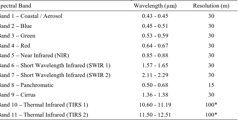
Landsat-8 satellite is a new Earth observing satellite launched on the 11th February, 2013. The sensors of Landsat-8 closely resembling its predecessor, Landsat-7, to ensure compatibility with historical data [14]. Its multispectral sensor, the operational land imager (OLI), is equipped with 9 reflective bands whereas the thermal infrared sounder (TIRS) is capable of measuring 2 emissive bands (Table 1).

Table 1: Landsat-8 band specifications. Bands 1-9 are OLI spectral bands while bands 10-11 are TIRS spectral bands.

Spectral Band Wavelength (µm) Resolution (m)

Band 1 – Coastal / Aerosol 0.43 - 0.45 30

* Bands 10 and 11 are resampled to 30 meter in delivered data products

Landsat-8 data of the central-west coast of peninsular Malaysia (path: 127 and row: 85), downloaded from the U.S. Geological Survey Earth Explorer website (http://earthexplorer.usgs.gov/), were used in this study. The data from 25th June, 2013, 8th March, 2014 and 25th April, 2014 were used to represent heavy, moderate and light hazy days respectively. Water bodies were not relevant to the analysis hence were masked out from the scene [5]. In-situ haze measurements in API (Air Pollution Index) used in this study were downloaded from the Department of Environment, Malaysia website (http://apims.doe.gov.my/apims). API is derived based on the concentration of the dominant air pollutants and the most dominant pollutant will represent the index of the day. In this study, the API measurements used are based on PM10.

2.2 HOT image derivation

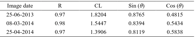
is established for each image [21]. To do so, clear pixels from each image are visually selected by inspecting the RGB (red, green and blue) composites of bands 4-3-2 and 5-4-3 for all images. Approximately 100 to 200 clear pixels are selected per image for deriving the CL. The DN value of each pixel is plotted on a scatter plot for band 4 against band 2 and the slope for the best-fit line is determined. The quality of the slopes is measured using coefficient of determination (R2). Selection process was repeated until the best R-value is achieved. Subsequently the slope is used to derive θ (arctangent of the slope), which is then used in equation (3). Here, B1 is the band 2 (blue) and B2 is band 4 (red) of Landsat-8. Table 2 summarises the coefficients required for deriving HOT images.

Table 2. Derived coefficients for HOT.

Image date R CL Sin (θ) Cos (θ) 25-06-2013 0.97 1.8204 0.8765 0.4815 08-03-2014 0.98 1.5447 0.8394 0.5434

25-04-2014 0.97 1.3906 0.8119 0.5838

2.3 API mapping

Linear regression was subsequently used to calibrate the HOT with the API values of the study area. In doing this, a 5×5 average filter window was used to sample training pixels above each API station to compensate for adjacency effect from neighbouring pixels. Accuracy of each regression model is determined by coefficient of determination (R2) (equation 4). Where n is the number of data points, i is the index of summation, APIcalculated is the calculated API from

regression equation, APImeasured is the measured ground-truth API, and APImean is

the mean of the APIcalculated.

Table 3. Regression equation R2 _{and RMSE for hazy, moderate and clear days.}

Image date API map equation R2 _RMSE

25-06-2013 _API_0.1036_HOT_589.91 0.2350 73.95 08-03-2014 API0.0135HOT23.34 0.2997 14.53 25-04-2014 _API_0.0054_HOT_23.22 0.1332 9.65

3 Results and discussion

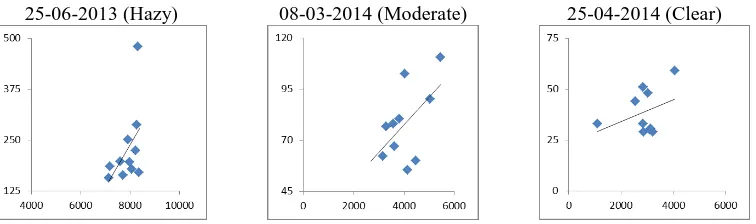
Linear regression plots between HOT and API are shown in Figure 2 while the corresponding regression equation, R2 and RMSE are given in Table 3. In overall, the outcome shows that based on the low R2 value, HOT is weakly correlated with API across different haze conditions. This is likely due to the quite lengthy gap between the API measurement and satellite overpass time. The satellite overpass time lags by approximately 30 minutes from the ground-truth measurement time hence the changes in haze concentration due to the dynamic atmospheric condition are likely to affect the haze estimation.

25-06-2013 (Hazy) 08-03-2014 (Moderate) 25-04-2014 (Clear)

Fig. 2. Scatterplots of API versus HOT and the regression lines for different hazy, moderate and clear days.

In Table 3, it is noticeable that RMSE increases as haze gets more severe with value of 9.65, 14.53 and 73.95 respectively. This may due to the different physical and chemical properties of the atmosphere during different haze conditions [15], [16]. PM10 particles, generally higher during hazy conditions than clear conditions,

Fig 3. RGB composite, HOT image and API map for hazy, moderate and clear day.

4 Conclusion

In this study, haze quantification from Landsat-8 using HOT technique has been studied. The result suggests that HOT is a practical technique to compute haze API spatially and continuously. Future research will focus on improving the accuracy by taking into account of meteorological and atmospheric factors to compensate for the time gap problem between satellite overpass and in-situ haze measurement.

Acknowledgements. We thank Universiti Teknikal Malaysia Melaka for funding this study under the UTeM Short Term Research Grant (UTeM PJP) (No.: PJP/2013/FTMK (4A)/S01146) and the Department of Environment, Malaysia for providing the API data.

References

[1] A. Ahmad and S. Quegan, Haze modelling and simulation in remote sensing satellite data, Applied Mathematical Sciences, 8(159) (2014), 7909–7921.

[2] A. Ahmad and M. Hashim, Determination of haze using NOAA-14 satellite data, Proceedings on The 23rd Asian Conference on Remote Sensing 2002 (ACRS 2002), (2012).

[3] A. Ahmad and M. Hashim, Determination of haze API from forest fire emission during the 1997 thick haze episode in Malaysia using NOAA AVHRR Data, Malaysian J. of Remote Sensing & GIS, 1 (2000), 77-84.

[4] A. Ahmad, M. Hashim, M.N. Hashim, M.N. Ayof and A.S. Budi, The use of remote sensing and GIS to estimate Air Quality Index (AQI) over Peninsular Malaysia, GIS development, (2006).

[5] A. Ahmad and S. Quegan, The effects of haze on the spectral and statistical properties of land cover classification, Applied Mathematical Sciences, 8(180) (2014), 9001–9013. http://dx.doi.org/10.12988/ams.2014.411939

[6] A. Ahmad, M.K.A. Ghani, S. Razali, H. Sakidin and N.M. Hashim, Haze reduction from remotely sensed data, Applied Mathematical Sciences, 8(36) (2014), 1755– 1762. http://dx.doi.org/10.12988/ams.2014.4289

[7] A. Ahmad, M. Hashim, N. Ayof, A.S. Budi, H. Sakidin and S.S. Ahmad, Determining of haze AQI over Malaysia using NOAA-14 AVHRR satellite data,

Pros. Persidangan Keb. Sains Matematik ke xiii, 1 (2005), 151-156.

[8] H. Sakidin, A. Ahmad and I. Bugis, Modelling of GPS tropospheric delay wet Neill mapping function (NMF), 3rd Int. Conference On Fundamental And Applied Sciences (ICFAS 2014), 3-5 June 2014, Kuala Lumpur, (2014).

http://dx.doi.org/10.1063/1.4898491

[9] J. Amanollahi, A.M. Abdullah, M.F. Ramli, and S. Pirasteh, Real time assessment of haze and PM10 aided by MODIS aerosol optical thickness over

Klang Valley, Malaysia, World Appl. Sci. J., 14 (2011), 8–13.

[10] M. Hashim, K.D. Kanniah, A. Ahmad, A.W. Rasib, Remote sensing of tropospheric pollutants originating from 1997 forest fire in Southeast Asia, Asian Journal of Geoinformatics 4 (2004), 57 – 68.

[11] M.S. Wong, J. Nichol, K.H. Lee, and Z. Li, Retrieval of aerosol optical thickness using MODIS 500 × 500m2_{, a study in Hong Kong and Pearl River delta}

region, Earth Obs. Remote Sens. Appl., (2008), 1-6. http://dx.doi.org/10.1109/eorsa.2008.4620353

In The North of Thailand and Chiang Rai Province, APCBEE Procedia 1, pp. 304–308, (2012). http://dx.doi.org/10.1016/j.apcbee.2012.03.050

[13] N.C. Hsu, M.J. Jeong, C. Bettenhausen, A.M. Sayer, R. Hansell, C.S. Seftor, J. Huang, and S.C. Tsay, Enhanced deep blue aerosol retrieval algorithm: The second generation, J. Geophys. Res. Atmos., 118 (2013), 9296–9315.

http://dx.doi.org/10.1002/jgrd.50712

[14] Q. Wang, Y. Zha, J. Gao, and D. Shen, Estimation of atmospheric particulate matter based on MODIS HOT, Int. J. Rem. Sens., 34(5), (2013), 1855–1865. http://dx.doi.org/10.1080/01431161.2012.730155

[15] U.S. Geological Survey, Landsat 8, USGS FS: 2013-3060, Reston, (2013). http://dx.doi.org/10.4135/9781452275956.n337

[16] J. Xu, X. Tai, R. Betha, J. He, and R. Balasubramanian, Comparison of physical and chemical properties of ambient aerosols during the 2009 haze and non-haze periods in Southeast Asia., Env. Geochem. Health, (2014).

http://dx.doi.org/10.1007/s10653-014-9667-7

[17] R. Betha, Z. Zhang, and R. Balasubramanian, Influence of trans-boundary biomass burning impacted air masses on submicron particle number concentrations and size distributions, Atmos. Env., 92 (2014), 9–18.

http://dx.doi.org/10.1016/j.atmosenv.2014.04.002

[18] Dept. of Environment Malaysia, Environmental Quality Report, (2005).

[19] R. Afroz, M.N. Hassan, and N.A. Ibrahim, Review of air pollution and health impacts in Malaysia, Environ. Res., 92(2), (2003), 71–77.

http://dx.doi.org/10.1016/s0013-9351(02)00059-2

[20] W.M.S. Wan Ahmad, Forest fire situation in Malaysia, Int. Forest Fire News No. 26, J.G. Goldammer, Ed. Geneva: FAO/ECE/ILO, 66–74, (2002).

[21] J.C. Keane, Air quality and visibility in southwestern British Columbia during forest fire smoke events, The Univ. of British Columbia, (2012).

[22] W.L. Chameides, H. Yu, S.C. Liu, M. Bergin, X. Zhou, L. Mearns, G. Wang, C.S. Kiang, R.D. Saylor, C. Luo, Y. Huang, A. Steiner, and F. Giorgi, Case study of the effects of atmospheric aerosols and regional haze on agriculture, Proc. Natl. Acad. Sci., 96(24) (1999), 13626–13633.

[23] Y. Zhang, B. Guindon, and J. Cihlar, An image transform to characterize and compensate for spatial variations in thin cloud contamination of Landsat images,

Remote Sens. Environ., 82 (2002), 173–187.

http://dx.doi.org/10.1016/s0034-4257(02)00034-2