CAUSAL AND DYNAMIC RELATIONSHIP AMONG STOCK RETURN, TRADING VOLUME, AND RETURN VOLATILITY IN SOUTH-EAST ASIA
MARKET PERIODS OF 2011-2014 Compiled by:
Harun
Student ID Number: 11 12 19348 Supervisor:
Prof., Dr., J. Sukmawati Sukamulja, MM. ABSTRACT
The purpose of this research is to examine the causal and dynamic relationship among stock market, trading volume, and return volatility in South-East Asia market period of 2011-2014. This research employs Vector Auto-Regression (VAR) and E-GARCH model. The causal and dynamic relationship between stock return and trading volume analyzed using VAR model, whereas dynamic relationship between return volatility and trading volume analyzed using E-GARCH model. Result showed that Thailand market return have no impact to trading volume, and vice versa. There is causal effect in Malaysia and Vietnam market. Stock return does not have impact to trading volume, but trading volume does have impact to return in Philippines and Indonesia. All countries in South-East Asia market indicated that trading volume information being useful in predicting future return volatility, except Philippines.
Keywords: Stock Return, Trading Volume, Return Volatility, VAR, E-GARCH
1. Introduction
price. The last reason, the relationship between stock return and trading volume has significant implications research into future market.
Thus, this research will examine the relationship among stock return, trading volume, and return volatility. This research picks evidence in South-East Asia stock market. Kirativanich (2000) concluded that South-East Asian Financial markets were attractive to investors looking for high returns on their investments. Both the financial and economic systems of South-East Asian had grown rapidly. Many investors thus began more favorably on and began investing in the South-East Asian financial market.
Therefore, investors need information about the place that have good prospect in the future. South-East Asian stock markets are one of other interesting stock markets. Investors also need information that can predict future price in order to get high return. Trading volume is a trigger that makes a stock price change. So, this research will investigate “Causal and Dynamic Relationship among Stock Returns, Trading Volume, and Return Volatility in South-East Asia Market Period of 2011-2014”.
2. Theoretical Background
The change of stock return is responded by investors. If the stock price decreases, investors are willing to buy the stock in hope will have return when the stock price up. If investors have stock with high price (overvalued), investors will sell the stock in order to get current return. It explained that the change of return have impact to trading volume. There are bidirectional relationship between stock return and trading volume. Trading volume has impact to stock return. On the contrary, the stock markets have impact to trading volume. Thus, there is causal relationship between stock return and trading volume.
H1 = There is causal and dynamic relationship among stock market returns, trading volume, and volatility in South-East Asia market period of 2011-2014
2 Research Method
3.1 Type of Methodology
Methodology is the guideline for fulfilling objectives of this research. This research employs Vector Auto-Regression (VAR) Model and Exponential-GARCH (EGARH). The VAR analysis is used to analyze the causality relationship between stock return and trading volume. The E-GARCH model is used to analyze the dynamic relationship between trading volumes and return volatility.
3.2 Sample
The sample of this research will take from composite indices of national stock market at South-East Asian; Indonesia, Singapore, Thailand, Philippine, Malaysia, and Vietnam. The sample used is monthly stock market indices data of those markets with time interval from May 2011 to December 2014. In this period, data of the six countries of South-East Asian are available. All data is taken from Yahoo Finance and Investing.com. These six stock exchanges are selected because the six countries have their stock market and historical data.
Table 3.1
List of Selected Stock Exchange and its Market Index
Country Name of Stock Exchange Name of Index
Indonesia Indonesia Stock Exchange (IDX) Jakarta Composite Index (JCI)
Malaysia Bursa Malaysia Stock Exchange Kuala Lumpur Composite Index (KLCI) Philippine Philippine Stock Exchange (PSE) Philippines Stock Exchange Index (PSEi) Thailand Stock Exchange of Thailand (SET) Bangkok Stock Exchange Index (BSEI) Vietnam Hanoi Stock Exchange Hanoi Stock Exchange Index (HNXI)
3.3 Research Variables
3.3.1 Measurement of Stock Return
Stock market return is taken from market index in each South-East Asia Country. Market index can represent of overall activity of each country. Market Return can be calculated by stock price in period t minus stock price index in period t-1 divided by stock price period t-1. Market return can be formulated mathematically as (Pisedtasalasai and Gunasekarage, 2008);
………...……… (1) where;
: Market Return in period t : Market Price in period t : Market Price in periodt-1 3.3.2 Measurement of De-trended Volume
The first variable of this research is return. According Choi et al (2012), trading volume has influence to return, and vice versa. To make regression model, these two variables should be in the same form. If the return is using percentage form, trading volume should be in the percentage form too. Thus, the form of trading volume will be formulated, as following (Pisedtasalasai and Gunasekarage, 2008);
……….…. (2)
where;
DVt = De-trended Volume in period t
Trading Volume t = Trading Volume in period t Trading Volume t-1 = Trading Volume in period t-1 3.4 Data Analysis Method
3.4.1 Vector Auto-Regression (VAR) Analysis
variable A have influence to variable B. while in the same, variable B also have influence to variable A. It means that there is causality relationship between variable A and variable B.
According Widarjono (2013), there are steps to run VAR analysis; (1) stationary test with the data, (2) Co-integration test, (3) determine maximum lag and optimal lag which will be used, (4) Causality test, (5) estimation VAR, and (6) analyze result of Impulse Response and Variance Decomposition.
1. Stationary Test
This research adopts a test for a unit root test to ensure that variable is stationary, and to avoid spurious regression (there is no relationship between dependent variable and dependent variable). Stationary test can detect spurious regression. Stationary test can explain the behavior of the data too. Therefore, it is important to stationary test for time series data.
The testing for a unit root is based on Augmented Dickey-Fuller (1979) (ADF) and Phillip-Perron (1988) (PP). ADF and PP test are used with trend and without trend. The ADF test formulated as follows (Widarjono, 2005);
………... (3)
Stationary data is based on statistical comparison from MacKinnon critical value. If statistic value of ADF and PP test absolutely higher that Mackinnon critical value in level α (1%, 5%, and 10%), so data is called stationary. Analyzing using VAR model, data used should be stationary in the same level. If one of data is not stationary, data should be tested in the 1st difference or 2nd difference.
2. Determining optimal lag
3. Estimation Vector Auto-Regression (VAR) Model
Estimation VAR model will used determined optimal lag based on five criteria that was mention above. Estimation VAR model can be investigated value of t-statistics in each variable. VAR model will be formulated by Ariefianto (2012) and adjusted with variables of this research. The formulation of the model is as follows;
Rt = α0 + + + εt………...…….….……. (4) DVt = λ0 + + + ηt……...……...……… (5) VAR model produce several important analysis; (2) Impulse Response, (3) Variance Decomposition, and (4) Granger Causality Test.
a. Impulse Response
It is difficult to interpret based on the coefficient of each variable, so econometricians use impulse response analysis. Impulse response is used to analyze the influence of a variable change to another variable dynamically. Impulse response works by giving shock for one endogen variable. Impulse response figures the path where a variable will be back to balance after shock happened from other variable.
b. Decomposition Variance
Beside impulse response, VAR model provide forecast error decomposition of variance known as variance decomposition. The purpose of decomposition variance is to predict the percentage of contribution variance in each variable because there is change of certain variable in VAR model (Juanda and Juanidi, 2012). Therefore, decomposition variance arranges approximate error variance of certain variable.
c. Granger Causality Test
Granger causality test analyze causal relationship between endogen variable in VAR model. Granger causality test indicate the relationship between variables is bidirectional or unidirectional. To examine causal relationship between trading volume, the following model estimated by Widarjono (2013);
………...…………..…. (6) ………..……….. (7)
equation (11) and (12) developed Granger Causality test hypothesis the following;
H01: Rt variable does not Granger cause another DVt H02: DVt variable does Granger cause another Rt 3.4.2 E-GARCH Model
The effect of trading volume on return volatilities analysis using first model the dynamic properties of the volatilities without the effect of trading volume. The following formulation leads to the asymmetric GARCH model, Exponential GARCH, of Nelson (1991) and adjusted with the research:
………... (8)
The research will use this formula to measure volatility. This formula explains the conditional variance respectively. The coefficient γ is an asymmetric effect of negative versus positive standardized residuals on conditional variances. A negative value of y means that negative residuals tend to produce higher conditional variances compared to positive one in the immediate future (Pisedtasalasai and Gunasekarage, 2008).
After the E-GARCH model is determined. The next step is diagnostic checking in the residual. The residual is desirable if there is no ARCH effect and the residual is normally distributed. ARCH-LM test will be used to check whether there is ARCH effect or not in the residual, whereas normality test is to check the residual whether the residual is normally distributed or not.
a. ARCH-LM Test
Engle developed a test to examine heteroskedasticity in times series data, known as Auto-Regressive Conditional Heteroskedasticity (ARCH) test. The basic idea of this test is the residual variance ( ) not only the function of independent variable, but also depends on Residual Square of the previous period (σ2
t-1) or can be written as follows (Widarjono, 2005):
If the value squares (x) are greater than critical value chi-square (x2) and probability value chi-squares (x) are less at the significant level 5%, it means that the model contains ARCH effect.
b. Normality Test
Normality test in residual can be detected using method developed by Jarque-Bera (JB). Jarque-Bera Method is to examine whether the residual is normally distributed or not. Jarque-Bera method measures skewness and kurtosis. The formulation statistically Jarque-Bera test is the following (Widarjono, 2005):
………. (11)
Where: S = Skewness K = Kurtosis
n = number of sample 3 Analysis Data
3.1 Descriptive Statistics
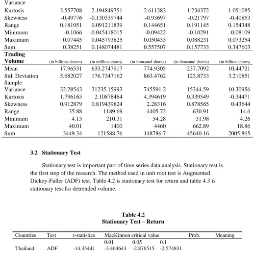
After all data are collected, descriptive statistics can be constructed based on weekly data of stock market returns and trading volume for five countries in South-East Asia; Thailand, Vietnam, Philippines, Malaysia, and Indonesia for period May 2011 to December 2014. The descriptive statistics reports the mean, standard deviation, skewness, kurtosis, and so on. The descriptive statistics will show the following table:
Table 4.1 Descriptive Statistics
Country Indonesia Malaysia Philippines Vietnam Thailand
Index Jakarta
Composite Index
Kuala Lumpur Composite Index
Philippines Stock Index
Vietnam Stock Exchange Index
Bangkok Stock Exchange Index Sample Period May 2011
-December 2014
May 2011 -December 2014
May 2011 -December 2014
May 2011 -December 2014
May 2011 –
December 2014
Observation 192 192 192 192 192
Return
Mean 0.001992 0.000771221 0.002904 0.000822 0.00181
Std. Deviation 0.02323 0.012665049 0.020767 0.030691 0.025508
Country Indonesia Malaysia Philippines Vietnam Thailand
Variance
Kurtosis 3.557708 2.194849751 2.611383 1.234372 1.051085
Skewness -0.49776 -0.130339744 -0.93697 -0.21797 -0.40853
Range 0.181051 0.091211839 0.144651 0.191145 0.154348
Minimum -0.1066 -0.045418015 -0.09422 -0.10291 -0.08109
Maximum 0.07445 0.045793825 0.050433 0.088231 0.073254
Sum 0.38251 0.148074481 0.557507 0.157733 0.347603
Trading
Volume (in billions shares) (in million shares) (in thousand shares) (in thousand shares) (in billion shares)
Mean 17.96531 633.2747917 774.9305 237.7092 10.44721
Std. Deviation 5.682027 176.7347162 863.4762 123.8733 3.210851
Sample
Variance 32.28543 31235.15993 745591.2 15344.59 10.30956
Kurtosis 1.796163 2.10878464 4.394619 0.339549 -0.34471
Skewness 0.912879 0.819439824 2.28316 0.878565 0.43644
Range 35.88 1189.69 4405.72 630.91 14.6
Minimum 4.13 210.31 54.28 31.98 4.26
Maximum 40.01 1400 4460 662.89 18.86
Sum 3449.34 121588.76 148786.7 45640.16 2005.865
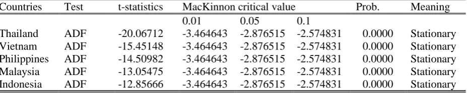
3.2 Stationary Test
Stationary test is important part of time series data analysis. Stationary test is the first step of the research. The method used in unit root test is Augmented Dickey-Fuller (ADF) test. Table 4.2 is stationary test for return and table 4.3 is stationary test for detrended volume.
Table 4.2
Stationary Test – Return
Countries Test t-statistics MacKinnon critical value Prob. Meaning
0.01 0.05 0.1
Thailand ADF -14.35441 -3.464643 -2.876515 -2.574831 0.0000 Stationary
Vietnam ADF -11.29448 -3.464643 -2.876515 -2.574831 0.0000 Stationary
Philippines ADF -13.58780 -3.464643 -2.876515 -2.574831 0.0000 Stationary
Malaysia ADF -14.06695 -3.464643 -2.876515 -2.574831 0.0000 Stationary
Indonesia ADF -15.32523 -3.464643 -2.876515 -2.574831 0.0000 Stationary
Table 4.3
Stationary Test – Detrended Volume
Countries Test t-statistics MacKinnon critical value Prob. Meaning
0.01 0.05 0.1
Thailand ADF -20.06712 -3.464643 -2.876515 -2.574831 0.0000 Stationary
Vietnam ADF -15.45148 -3.464643 -2.876515 -2.574831 0.0000 Stationary
Philippines ADF -14.50982 -3.464643 -2.876515 -2.574831 0.0000 Stationary
Malaysia ADF -13.05475 -3.464643 -2.876515 -2.574831 0.0000 Stationary
Indonesia ADF -12.85666 -3.464643 -2.876515 -2.574831 0.0000 Stationary
This stationary test for both return and detrended volume data series indicate stationary in Level (0). The first difference level of stationary test is not needed. Return and detrended is not contained unit roots, thus the following process could be conducted which is estimation VAR model.
3.3 VAR Model
4.3.1 Determining Optimal Lag
To employ Vector Auto-Regression (VAR) model, determining the lag length is important. Determining the lag can be done by using Lag Order Selection Criteria VAR test. The optimal lag can be determined based on some indicators such as Akaike Information Criterion (AIC), Schwartz Information Criterion (SIC), Hannan-Quinn Criterion (HQ), Likelihood Ratio (LR), and Final Prediction Error (FPE). The optimal lag order selected based on the lowest number of all criterion.
Table 4.4
VAR Lag Order Selection Criteria
Country Optimal Lag
Thailand 1
Vietnam 3
Philippines 2
Malaysia 5
Indonesia 2
4.3.2 VAR Estimation
is no spurious regression. The estimation result of VAR model shows in the following table;
Table 4.5
Vector Auto-Regression Model
Country Thailand Vietnam Philippines Malaysia Indonesia Panel A: estimation equation 4
Lag (k) 1 3 2 5 2
F-statistics 0.522387 2.738598** 0.317022 1.998274* 1.233069 R-squared 0.005527 0.082807 0.006808 0.101962 0.025969 AIC -4.490101 -4.154604 -4.870744 -5.884901 -4.656191 SIC -4.439019 -4.034539 -4.785296 -5.694836 -4.570743 Panel B: estimation equation 5
Country Thailand Vietnam Philippines Malaysia Indonesia
F-statistics 0.350927 2.022106* 7.711941** 4.615053** 3.937583** R-squared 0.131886 0.062497 0.142914 0.207744 0.511680 AIC 0.759105 1.877695 1.363532 0.370216 0.511680 SIC 0.810188 1.997760 1.448980 0.560281 0.597128 Note: Standard errors in ( ) & t-statistics in [ ], An ∗,∗∗ denotes statistical
significance at the 5%, 1% level
Table 4.5 presents causality test results obtained through the estimation of VAR models using equation 4 and 5 (see chapter 3). Panel A reports the results from equation 4 when Rt is the dependent variable while panel B reports the results from equation 5 when DVt is the dependent variable.
Estimation Vector Auto-Regression (VAR) model concluded that Thailand market return have no impact to trading volume, and vice versa. It is different with Vietnam market, the stock market return in Vietnam have impact to trading volume, and vice versa. Stock return does not have impact to trading volume, but trading volume does have impact to return in Philippines, Malaysia, and Indonesia.
4.3.3 Causality Test
Table 4.6
Granger Causality Tests
Countries Lags Null Hypothesis: Obs F-Statistic Prob. Meaning
Thailand 1 DV does not Granger Cause R 191 0.80706 0.3701 Ho: supported
R does not Granger Cause DV 0.21205 0.6457 Ho: supported
Vietnam 3 DV does not Granger Cause R 189 1.72684 0.1631 Ho: supported
R does not Granger Cause DV 3.01908 0.0312 Ho: not supported
Philippines 2 R does not Granger Cause DV 190 0.33670 0.7146 Ho: supported
DV does not Granger Cause R 0.33191 0.7180 Ho: supported
Malaysia 5 DV does not Granger Cause R 187 3.01661 0.0122 Ho: not supported
R does not Granger Cause DV 2.11700 0.0655 Ho: not supported
Indonesia 2 DV does not Granger Cause R 190 1.02260 0.3617 Ho: supported
R does not Granger Cause DV 0.15109 0.8599 Ho: supported
The results of Granger Causality test conclude that Thailand, Philippines, and Indonesia have no causal relationship between trading volume and stock market return. There is unidirectional relationship between trading volume and stock market return in Vietnam. The stock market returns of Vietnam have impact to detrended volume, but it not in reverse. It may indicate that there is causal relationship between stock return and trading in longer period. The causal (bidirectional) relations between trading volume and stock market return in Malaysia. The detrended volume has impact to stock market return, and vice versa.
4.3.3 Impulse Response
-.01 Response of R to DV
-.2 Response of DV to R
-.2 Response of DV to DV Response to Cholesky One S.D. Innovations ± 2 S.E.
Thailand Response of R to DV
-.2 Response of DV to R
-.2 Response of DV to DV Response to Cholesky One S.D. Innovations ± 2 S.E.
-.4 Response of DV to DV
-.4 Response of DV to R
-.004 Response of R to DV
-.004 Response to Cholesky One S.D. Innovations ± 2 S.E.
-.01 Response of R to DV
-.2 Response of DV to R
-.2 Response of DV to DV Response to Cholesky One S.D. Innovations ± 2 S.E.
-.004 Response of R to DV
-.2 Response of DV to R
-.2 Response of DV to DV Response to Cholesky One S.D. Innovations ± 2 S.E.
Graph 1 Impulse Response
In Thailand, stock market returns have move up in the beginning period because of shock from detrended volume, but it is in small number. The value of stock market return will be 0.0015544 if stock market return got a shock from detrended volume. It can be seen in first period. There is no significant change because of shock of stock market return to detrended volume. The value of detrended will be 0.009244 when detrended volume got a shock from stock market return in the second period.
The response of stock market return is increasing in beginning up to period 3. It is back to zero again in the period 5. When stock market return got shock from detrended volume, the value of return will be 0.003829 in third period as the highest change. The change because of shock from detrended volume is high. The fluctuation of detrended volume happens because of shock from the stock market return. Because of shock from return, the value of detrended volume is 0.0090582 in the first period and fall down to -0.095228 in the fourth period.
The interesting part of Malaysia, both variables, return and detrended volume move fluctuated. The response of return is in the fourth and fifth period with the value is 0.002138 and 0.002143. Whereas response of detrended volume, the value of detrended volume is -0.046429 in first period. There are two peak of response of detrended volume which is in fourth and sixth period with the values are 0.030366 and 0.043889
In Indonesia, stock market returns increase up to 0.002052 in the third period. It is the highest response of return. In the beginning of period, because of return shock, the value of detrended volume is 0.308139. In the rest period, there is no highly response of detrended volume.
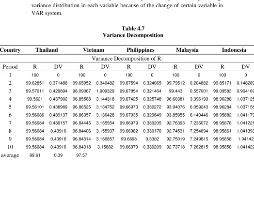
4.3.5 Variance Decomposition
Impulse response analysis is used to track the shock of variable to other variable, while variance decomposition analysis is to predict the percentage variance distribution in each variable because of the change of certain variable in VAR system.
Table 4.7
Variance Decomposition
Country Thailand Vietnam Philippines Malaysia Indonesia
Variance Decomposition of R:
Period R DV R DV R DV R DV R DV
1 100 0 100 0 100 0 100 0 100 0
2 99.62851 0.371488 99.65952 0.340482 99.67594 0.324065 99.79512 0.204882 99.85171 0.148289 3 99.57011 0.429894 98.09067 1.909329 99.67854 0.321464 99.443 0.557001 99.09583 0.904169 4 99.5621 0.437902 96.85568 3.144318 99.67425 0.325748 96.60381 3.396193 98.96288 1.037125 5 99.56101 0.438989 96.86525 3.134752 99.66973 0.330272 93.94076 6.059243 98.96284 1.037158 6 99.56086 0.439137 96.86357 3.136428 99.67035 0.329649 93.85955 6.140446 98.95882 1.041179 7 99.56084 0.439157 96.84445 3.155554 99.66979 0.330205 92.76393 7.236072 98.95878 1.041221 8 99.56084 0.43916 96.84406 3.155937 99.66982 0.330176 92.74531 7.254694 98.95861 1.041393 9 99.56084 0.43916 96.84314 3.156857 99.6698 0.3302 92.75019 7.249815 98.95858 1.04142 10 99.56084 0.43916 96.84318 3.15682 99.66979 0.330209 92.73718 7.262815 98.95858 1.041422 average 99.61 0.39 97.57 2.43 99.7 0.3 95.46 4.54 99.17 0.83
Variance decomposition of DV:
Period R DV R DV R DV R DV R DV
Country Thailand Vietnam Philippines Malaysia Indonesia 4 0.102821 99.89718 6.300942 93.69906 1.816226 98.18377 3.808989 96.19101 0.316353 99.68365 5 0.102976 99.89702 6.303300 93.69670 1.827301 98.1727 4.312939 95.68706 0.316376 99.68362 6 0.102997 99.8970 6.336178 93.66382 1.828505 98.1715 6.157007 93.84299 0.316535 99.68347 7 0.103001 99.8970 6.352803 93.6472 1.828932 98.17107 6.307311 93.69269 0.316532 99.68347 8 0.103001 99.8970 6.360071 93.63993 1.82923 98.17077 6.306237 93.69376 0.316546 99.68345 9 0.103001 99.8970 6.361252 93.63875 1.829231 98.17077 6.360762 93.63924 0.316547 99.68345 10 0.103001 99.8970 6.361577 93.63842 1.829262 98.17074 6.382592 93.61741 0.316548 99.68345 average 0.09518 99.90482 5.449716 94.55029 1.784364 98.21564 4.800092 95.19991 0.296347 99.70365 Source: appendix 8
Table 4.7 presents the variance decomposition of return and trading volume in the period 1-10. The average variance decomposition of return is 0.39%, 2.43%, 0.3%, 4.54%, and 0.83% explained by trading volume for Thailand, Vietnam, Philippines, Malaysia, and Indonesia. The average variance decomposition of trading volume can be explained by return 0.095%, 5.45%, 1.78%, 4.8%, and 0.296% for Thailand, Vietnam Philippines, Malaysia, and Indonesia.
4.4 E-GARCH Model
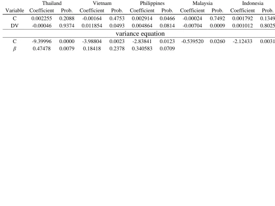
4.4.1 Estimates of E-GARCH Model
Table 4.8 reports the estimated parameters of the EGARCH model with asymmetric effect for each market given by equation 11. There are three points that can be analyzed (1) leverage effect, (2) time varying volatility, and (3) the ability of detrended volume to predict the future dynamics of return volatilities. To examine whether there is asymmetric effect in stock market return showed in coefficient of γ. If the coefficient of γ is negative and statistically significant in the 5% level concluded that there is asymmetric effect in the model of return volatility. To examine whether there is time varying volatility by concerning to coefficient of α. Then, analyzing the predictive power of trading volume to forecast the future dynamic return volatility can be seen in the coefficient of detrended volume.
Table 4.8
Estimates of E-GARCH Model
Thailand Vietnam Philippines Malaysia Indonesia
Variable Coefficient Prob. Coefficient Prob. Coefficient Prob. Coefficient Prob. Coefficient Prob.
C 0.002255 0.2088 -0.00164 0.4753 0.002914 0.0466 -0.00024 0.7492 0.001792 0.1349
DV -0.00046 0.9374 0.011854 0.0493 0.004864 0.0814 -0.00704 0.0009 0.001012 0.8025
variance equation
C -9.39996 0.0000 -3.98804 0.0023 -2.83841 0.0123 -0.539520 0.0260 -2.12433 0.0031
0.47478 0.0079 0.18418 0.2378 0.340583 0.0709 0.016984 0.8568 0.60938 0.0000
-0.12361 0.1661 0.13585 0.1942 -0.25307 0.0071 -0.280520 0.0004 -0.23688 0.0050
α -0.21106 0.2523 0.471103 0.0106 0.674462 0.0000 0.945677 0.0000 0.793698 0.0000
DV 0.52486 0.0332 0.770106 0.0003 0.024587 0.9430 1.269540 0.0000 0.948172 0.0013
4.4.2 ARCH LM Test
The heteroskedascity test is to examine the residuals is containing heteroskedascity or not. This test would be performed by ARCH LM test. The result of heteroskedascity showed in the following table:
Table 4.9 ARCH LM Test
Country Obs*R-squared Prob. Chi-Square (1)
Thailand 0.170633 0.6795
Vietnam 0.135616 0.7127
Philippines 0.096971 0.7555
Malaysia 0.077431 0.7808
Indonesia 0.001148 0.9730
4.4.3 Normality Test
Table 4.10 Normality Test
Country Skewness Kurtosis Jarque-Bera Probability
Thailand -0.514982 3.980944 16.18460 0.000306
Vietnam -0.576437 4.093170 20.19314 0.000041
Philippines -0.665329 4.168115 25.08117 0.000004
Malaysia -0.046385 3.093756 0.139170 0.932781
Indonesia -0.330796 3.486723 5.396828 0.067312
The null hypothesis is data normally distributed. The alternative hypothesis is data not normally distributed. The null hypothesis is supported if the p-value is greater than significant level 5%. Look at, table 4.10, there are two residual models are normally distributed that is Malaysia and Indonesia. The residual of others countries is not normally distributed.
4.5 Conclusion
This research analyzed causal and dynamics relationship among stock return, return volatility, and trading volume in South-East Asia Market. The result of this research be concluded that Thailand market return have no impact to trading volume, and vice versa. It is different with Malaysia and Vietnam market, the stock return have impact to trading volume, and vice versa. Stock return does not have impact to trading volume, but trading volume does have impact to return in Philippines and Indonesia. All country in South-East Asia market indicates that trading volume information being useful in predicting future return volatility, except Philippines.
References
Aggarwal, R., Inclan, C., and Leal, R., (1999), Volatility in Emerging Stock
Markets, The Journal of Financial and Quantitative Analysis, Vol. 34, No.
1, pp. 33-55
Ariefianto, M.D., (2012). Ekonometrika: Esensi dan Aplikasi dengan Menggunakan Eviews, Penerbit Erlangga
Asghar, N., (2011), “The Empirical Relationship between Stock Returns and Trading Volume in Pakistan (2000-2006)”, Interdisciplinary Journal of Contemporary Research in Business, Academic Journal, June, Vol. 3, p1356 Assan A. and Thomas S., (2013), “Stock returns and trading volume: does the size matter?”, Investment Management and Financial Innovations, Volume 10, 76-88
Bodie, Z., Kane A., and Marcus J.A., (2006), Investment, 6th Edition, McGraw-Hill
Bodie, Z., Kane, A., and Marcus J.A., (2010), Essentials of Investment, Ninth Edition, McGraw-Hill
Brealey, R.A., Myers, S.C., and Marcus, A.J. (2001), Fundamental of Corporate Finance, Third Edition, McGraw-Hill
Chiang, T.C., and Doong, SC., (2001), “Empirical Analysis of Stock Returns and Volatility: Evidence from Seven Asian Stock Markets Based on TAR-GARCH Model”, Review of Quantitative Finance and Accounting, 17: 301– 318,
Countries of South-East Asia, Retrieved September 2015, from Northern Illinois University: www.niu.edu
Darwish, M.J., (2012), “Testing the Contemporaneous and Causal Relationship between Trading Volume and Return in the Palestine Exchange”. Interdisciplinary Journal of Contemporary Research in Business, Vol 3, No 10
Fama, E.F., (2010). “Efficient Capital Markets: A Review of Theory and Empirical Work”. Blackwell Publishing for the American Finance Association, Papers and Proceedings of the Twenty-Eighth Annual Meeting of the American Finance Association New York, Journal of Finance, Vol. 25, No. 2
Grossman, S.J. and Stiglitz, J.E., (1980), “On the Impossibility of Informationally Efficient Markets”, The American Economic Review, Vol. 70, No. 3
Habib, N.M., (2011), “Trade Volume and Returns in Emerging Stock Markets An Empirical Study: The Egyptian Market”, International Journal of Humanities and Social Science, December, Vol. 1, No. 19
Hartono, J., (2010), Teori Profolio dan Analisis Investasi, eighth edition, Yogyakarta: Badan Penerbit Fakultas Ekonomi Universitas Gadjah Mada Jiang, W., (2012), “Using the GARCH model to analyze and predict the different
stock markets”, Master Thesis in Statistics, Department of Statistics, Uppsala University, Sweden
Kirativanich, T., (2000), “The Effects of Macroeconomic Variables on the Southeast Asian Stock Market: Indonesia, Malaysia, the Philippines, and Thailand”, Dissertation Presented to the Graduate Faculty of the College of Business Administration United States International University
Kiymaz, H., and Girard, E., (2009), “Stock Market Volatility and Trading Volume: An Emerging Market Experience”, the ICFAI Journal of Applied Finance, Vol. 15, p. 5-32
Lee, M.C.M., and Swaminathan, B., (2000), Price Momentum and Trading Volume, the Journal of Finance, Vol. LV, No. 5
Leon, N.K., (2007), “An empirical study of the relation between stock return volatility and trading volume in the BRVM”, Academic Journals; African Journal of Business Management Vol. 1 (7), pp. 176-184,
Liaw, K.T., (2004), Capital Market, Thomson-Learning, South-Western, United States of America
Marusiakova, M., (2006), Forecasting Financial Market Volatility, Department of Probability and Mathematical Statistics Charles University, Prague
Mestel, R., Gurgul, H., and Majdosz, P., (2003) “Joint Dynamics of Prices and Trading Volume on the Polish Stock Market”, Managing Global Transitions 3; Vol. 3, No. 2
Mubarik, F., and Javid, A.Y., (2009), “Relationship between Stock Return, Trading Volume, and Volatility: Evidence from Pakistani Stock Market”, Asia Pacific Journal of Finance and Banking Research, Vol. 3, No, 3
Murphy, J.J., (1999), Technical Analysis of the Financial Markets: A Comprehensive to Trading Methods and Applications, New York Institute of Finance
Odean, T., (1998), Are Investors Reluctant to Realize Their Losses?, The Journal of Finance, October, Vol. LIII, No. 5
Odean, T., (1999), Do Investors Trade Too Much, the American Economic Review, December, Vol. 89, No. 5
Oral, E., (2012), “An empirical analysis of trading volume and return volatility relationship on Istanbul stock exchange national -100 Index”, Journal of Applied Finance & Banking, vol.2, no.5, 149-158
Pisedtasalasai, A. and Gunasekarage, A., (2008), “Causal and Dynamic Relationships among Stock Returns, Return Volatility and Trading Volume: Evidence from Emerging markets in South-East Asia”, Springer Science and Business Media, Asia-Pacific Finance Markets, 14, 277-297
Poon, S.H., and Granger, C.W.J., (2003), “Forecasting Volatility in Financial Markets: A Review”, Journal of Economic Literature, Vol. XLI, pp. 478– 539
Ross, S.A., Weterfield, R.W., and Jordan B.D., (2010), Corporate Finance Fundamentals, Eighth Edition, McGraw-Hill
Saunders, A. and Cornett, M.M., (2012), Financial Institution Management: A Risk Management Approach, Eighth Edition, McGraw-Hill
Van Horne, J.C., and Wachowhicz J.R., (2005), Fundamentals of Financial Management, twelfth edition, Prentice Hall
Wennstrom, A., (2014). “Volatility Forecasting Performance: Evaluation of GARCH type volatility models on Nordic equity indices”, Master of Science Thesis, Department of Mathematics, Royal Institute of Technology (KTH), Stockholm, Sweden
Widarjono, A., (2013). Ekonometrika: Pengantar dan Aplikasinya, Disertai Panduan Eviews, Fourth Edition, UPP STIM YKPN