CLASSIFICATION OF ARM MOVEMENT BASED ON UPPER LIMB MUSCLE SIGNAL FOR REHABILITATION DEVICE.

(1)

CLASSIFICATION OF ARM MOVEMENT BASED ON

UPPER LIMB MUSCLE SIGNAL FOR REHABILITATION

DEVICE

1_M.H.JALI,2_{’I.M.IBRAHIM,}3_Z.H.BOHARI,4_M.F.SULAIMA,5_M.N.M.NASIR

Faculty Electrical Engineering, Universiti Teknikal Malaysia Melaka, MALAYSIA

E-mail: 1mohd.hafiz@utem.edu.my, 2' iffamastura@gmail.com, 3zulhasrizal@utem.edu.my ,

4

fani@utem.edu.my , 5mohamad.naim@utem.edu.my

ABSTRACT

Rehabilitation device is used as an exoskeleton for people who experience limb failure. Arm rehabilitation device may ease the rehabilitation programme for those who suffer arm dysfunctional. The device used to facilitate the tasks of the program should improve the electrical activity in the motor unit by minimising the mental effort of the user. Electromyography (EMG) is the techniques to analyse the presence of electrical activity in musculoskeletal systems. The electrical activity in muscles of disable person are failed to contract the muscle for movements. To prevent the muscles from paralysis becomes spasticity or flaccid the force of movements has to minimise the mental efforts. To minimise the used of cerebral strength, analysis on EMG signals from normal people are conducted before it can be implement in the device. The signals are collect according to procedure of surface electromyography for non-invasive assessment of muscles (SENIAM). The implementation of EMG signals is to set the movements’ pattern of the arm rehabilitation device. The filtered signal further the process by extracting the features as follows; Standard Deviation(STD), Mean Absolute Value(MAV), Root Mean Square(RMS), Zero Crossing(ZCS) and Variance(VAR). The extraction of EMG data is to have the reduced vector in the signal features for minimising the signals error than can be implement in classifier. The classification of features is by SOM-Toolbox using MATLAB. The features extraction of EMG signals is classified into several degree of arm movement visualize in U- Matrix form.

Keywords: Arm Rehabilitation Device, Electromyography, Self-Organizing Map, Time Domain Features Extraction, Exoskeleton

1. INTRODUCTION

Human support system is known as an endoskeleton. Endoskeleton plays a role as a framework of the body which is bone. Our daily movements are fully depends on the functionality of our complex systems in the body. The disability one or more of the systems in our body will reduce our physical movements. Exoskeleton device is known as rehabilitation device to facilitate disable person. The functionality of the rehabilitation device has to smooth as the physical movement of normal human.

People who have temporary physical disability have the chances to recover. The rehabilitation programs provide the suitable plan for conducting the nerve and stimulate the muscles. Nowadays, rehabilitation program are using rehabilitation devices in their tasks. The

functionality of devices depends on muscle contraction. Electromyogram studies help to facilitate the effectiveness of the rehabilitation device.

(2)

2. SIGNAL PROCESSING the desired output. EMG signal is one type of bio signal that contains lot of noise from many factors. The noise may come from the skin at the electrode placement, type of electrode that may use for data collecting and also the environment. There are various type of size and pattern of electrodes, depends on the muscle area would like to detect and the thickness of the skin layer. The EMG noise signal can be reduced by choosing the gelled electrode which were Silver –Silver Chloride(AgCl) as the substance. Ag-AgCl introduces less electrical noise into the measurements. However, these noise should be eliminate to have a better signal for analysing purpose, the noise can be eliminate by many factors such as control environment, electrode placements and signal acquisition circuitry and configuration [1][2]. As for the features extraction there were various types in terms of frequency domain, time frequency domain and time scale domain. These types are chose based on the purpose of the analysis of the signal. In signal conditioning for time domain analysis, there is some features that can be applied. These features are described briefly as follows:

i) Root-Mean-Square (RMS)

RMS is the square root of the mean over time of the square of the vertical distance of the graph from the rest state. It much related to the constant force and non-fatiguing contraction of the muscle. In most cases, it is similar to standard taking the average of the absolute value of EMG signal. Since it represents the simple way to detect muscle contraction levels, it becomes a popular feature for deviation is calculated as the square root of variance.

The Artificial Neural Network(ANN) analysis is one of the computer science’s branch. The ANN’s are significant in problem solving such as pattern recognition and classification. ANN analysis is a dominant tool to analyze data and to interpret the results of the analysis, followed by sketching the conclusions on a structure of analyzed data. Self-organizing map(SOM) is well known as one type of neural network model that were commonly used for visualizing the data and to cluster the data. SOM was introduced by T. Kohonen in 1982, his exploration into this model to preserve the topology of multidimensional data. SOM is learns as unsupervised manner, which means no human intervention is needed throughout the learning. The SOM is a bundle of nodes, attached to one another via a rectangular or hexagonal topology in Figure 1 [10].

(3)

The learning starts from the components of the vectors Mij initialized at random. If n-dimensional vectors X1, X2,..., Xm are needed to map, the components of these vectors x1, x2, ..., xn are passed to the network as the inputs, where

m is the number of the vectors, n is the number

of components of the vectors. At each learning step, an input vector Xp ϵ {X1, X2, ..., Xm } is passed to the neural network. The vector Xp is compared with all the neurons Mij. Regularly the Euclidean distance || Xp – Mij || between the input vector Xp and each neuron Mij is calculated. The vector (neuron) Mc with the least Euclidean distance to Xp is elected as a winner [3][4].

Training the SOM network after carrying out the learning step is to evaluate the quality of the learning. Two types of errors which are; topographic error, Ete and quantization error, Eqe are calculated. The quantization error Eqe shows how well neurons of the trained network adapt to the input vectors. Quantization error (1) is the average distance between the data vectors Xp and their neuron-winners Mc(p) [11].

∑

(4)

Meanwhile the topographic error Ete shows how well the trained network keeps the topography of the data analyzed. The topographic error (2) is calculated by the formula:

∑

(5)

The distance of the neighbouring neurons can be visualized by using the visualization technique so-called unified distance matrix (U-matrix). U-matrix shows the distance of neighbouring neurons and the number of neighbours. The SOM is visualized by u-matrix as presented in Figure 2.

Figure 2: U-Matrix Representations In SOM

Figure 3: The Features’ Distance In Their Own Class Of Features.

(4)

software. Pavel Stefanoviˇ et al. investigation in his study proved that SOM-Toolbox had most advantages of possibilities such as:

i. Amount of data items and dimensions.

ii. Represent class names of all neuron winners in the same cell of map. iii. Easy data file preparation.

iv. Represents distance between neurons in a map.

v. Can be used some neighbouring function and any learning rate. vi. Can be used different learning step

(epochs or iterations).

SOM-Toolbox has a lack of losing the possibility for represent proportion of different classes of neuron winners in the cell of a map. The new system of SOM is the only model has this possibility, which previously improved.

4. EXPERIMENTAL SETUP

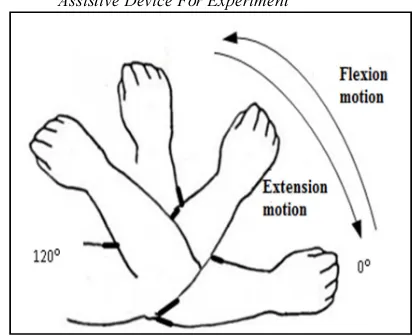
The experiment’s environment is in a room with low lighting especially the fluorescent light, any electromagnetic devices is away from the experiment equipment and the environment is in soundless room. Then, the experimental is set up with the subject sit on the chair while the hand is on the table. The subject has to complete the task of lift up the dumbbell with 2.27kgs of weigh in Figure 5 for 10 times. Mostly, the EMG signal is obtained after several trials of the movements. Normally, the appearance of EMG signal is chaos and noisy depends on the type of electrodes also the noise factor. To simplify the difference of amplitude response’s motion, the dumbbell is functioned to amplify the amplitude in analyzing the electrical activity during rest and contract. The rehabilitation devices(white in colour on Figure 4) helps to keep the position of the elbow joint and the wrist joint in line without being affected by the weight of the dumbbell during lift up motion. These movements are specified from angle of 0°(arm in rest position), up to 120°(arm is fully flexion) [6][7]. The experiment will go through several phases as explained in the next section [8].

Figure 4: Subject Is Set-Up With Arm Rehabilitation Assistive Device For Experiment

Figure 5: Simulation Of Subject Has To Lift Up The Dumbbell 2.27 Kgs Of Weight

i. Phase 1: Skin Preparation and Electrode

Placements.

(5)

collect the data. The combination of Arduino Mega and the OLIMEX shield, simplified the hardware. As the EMG signals are too sensitive towards magnetic devices, the neatness of the hardware is needed. The neatness ensured the electrode leads and the detecting surface intersects most of the same muscle on subject as in Figure 7(b) at biceps, and as a result, an improved superimposed signal is observed. Reference electrode has to be at the body where no muscles exist as the ground signal, for this experiment it placed at wrist on the unaffected hand(refer 7(b)).

(a) (b)

Figure 6: The Alcohol Swab(a) And The Gelled Electrode(b) That Used In This Experiment.

ii. Phase 2: sEMG Signal Acquisition

(a) (b)

Figure 7: The Biceps Brachii Muscles For Electrode Positions(a), The Electrode Placements On Subject

Skin(b)

Gelled electrode has two leads detecting surfaces and one lead as reference electrode. These two detecting surface need to be placed in range of less than 1-2 cm from each of it at the biceps muscle as in Figure 7(b). The gelled electrode for the blue lead and red lead are placed at the biceps skin for detection purpose, meanwhile the gelled electrode with black lead is placed at area with no muscles exist and unaffected hand.[1] The grounded electrode hand is placed at the leg to have a better grounding purpose. From Figure 8 these EMG signals will go through into high voltage protection to protect any electrical surge that may bring harm to the user and the hardware. These signals are available for signal conditioning process as the next step to be taken. The circuit that be used in this experiment is provided by the OLIMEX shield. The signals via the OLIMEX shield through the analogue circuit are very weak the voltage is around 10μV, full of noise and contain primarily 60Hz of frequency. The signals are next need to be filter and rectify, reducing the noise and amplifying the signals for analysis purpose. After the signals is filtered and amplified the signals is sent to the digital board and yet ready to display into the MATLAB software [9].

(6)

Figure 8: The Electrical Diagram Of Electrode Sensor, High Voltage Protection And Frequency

Rejection.

iii. Phase 3: Signal Conditioning

The signals from the board are gathered in the SIMULINK software. Signals from the OLIMEX shield need to be filtered by using the peak notch filter and the high pass filter. Peak notch filter is used for filtering the interference from the line AC and radio frequency from the devices frequency nearby. Meanwhile, the high pass filter is used for placed the baseline of EMG signals display in the scope(SIMULINK) at the zero line, also known as DC offset. Block diagram for collecting the EMG signal is showed in Figure 9. The raw EMG signals is next to filter by using Butterworth filter. The Butterworth filter is set to 5th order and 10/1000 Hz frequency. The filtered signal is accessed for features extraction. This EMG signal evaluated in time domain features. The analysis of this study soon to be applies in real-time application. Thus, the time-domain suits this study for better future work. These features are Root-Mean-Square(RMS), Mean Absolute Value(MAV), Standard Deviation(STD), Variances(VAR), and Zero Crossing(ZCS). This statistical information of the features evaluations were run in the MATLAB R2013a. The signals that gathered from the SIMULINK is next to be apply for features extraction. The features are extracted using MATLAB 2013a programming.

Figure 9: Block Diagram In SIMULINK Software For Collecting The EMG Signals.

iv. Phase 4: Signal Classification

Subsequently, the EMG features is analysed for classification process. The features are to be chose either it suits in classification process or not. The classification process is conducted by using unsupervised artificial neural network technique, which is Self-Organizing Map(SOM). The SOM is simulated using MATLAB software to classify the angle movement of the subjects. This is to achieve the objective of this study which is to classify the extracted features of EMG signal base on the angle movement. The classification signal can be further analyse for arm rehabilitation device implementation.The SOM-Toolbox need the user to organize the data(features) in column form to be analysed. The user also needs to set up the number of neuron to be use in the analysis. This number of neuron is important to determine the training time, size of map, and the error. Then, the data were called to run the analysis. From the analysis, the SOM-Toolbox gave the number of two types of error, quantization error and topographic error. The analysis through the SOM is recorded. The recorded analysis is next to be proved by the features either the pattern is recognized by the features or unrecognized and yet this study cannot be proved.

5. RESULTS AND DISCUSSIONS

(7)

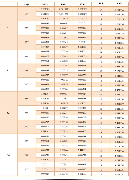
movement. However, to simplify the data input into the ‘m.file’, the data is calculated to average value for each movement. The simplified table is represented in Table 1.

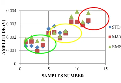
ZCS and VAR formed the absolute and 10-6 scientific number that would not achievable to be class into the classifier because of the distance of features itself. Data from Table 1 is plotted into scatter graph in Figure 10. Sample 1 up to sample 4 be owned by movement of 60˚, sample 5 to sample 8 is belong to movement of 90˚ and sample 9 to sample 12 is fit in movement 120˚. The green, yellow and red outline colour in Figure 10 shows that the scatter features is obviously been clustered by its angle of movements’ class. Even though the clustered movements is scattered in its class, the objective of this study is achievable. The learning of the features is continued in data classification. Thus, the ZCS and VAR are the features that have been eliminated in SOM classification technique.

Figure 10: The Scatter Graph Of Features Versus Amplitude Voltage.

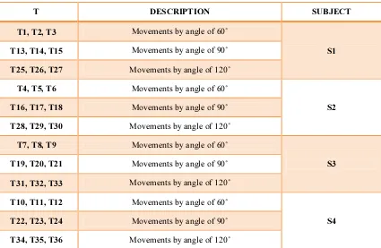
The unsupervised manner is applied in SOM-Toolbox using MATLAB software. This toolbox is a powerful tool that may helps to cluster randomized data. The data can be cluster even though the data is not arranged on its class. The more data the merrier clustering process. The data from Table 1 is relabelled into predefine ‘T’. Ts are defined as the trials belong to movements for certain angle in Table 2. Its’ labelled as predefined T in ‘m.file’ in MATLAB for data training. The random data training is compiled in ‘m.file’ and number of neuron is update to observe the clustered data of predefine ‘T’.

The data training is started by 100 of neurons. SOM-Toolbox visualized the output as in Figure 11(a)(b). Figure 11(a) shows the component planes in SOM. The variables in component planes are the features of EMG signal for all subjects. The features are RMS, MAV and STD. The components by each variable shows that the feature is clustered on its own feature class. In MAV feature plane shows that the MAV data is clustered at the top left of the plane. Which means the clustered data in dark blue colour is clustered and the distance among the data is closed. The dark blue colour in MAV plane is surrounded by the light blue, green, yellow and red colour. The colour in the plane shows the distance from the components that had cluster. The red colour is the farthest distance from the clustered data. RMS shows quite similar clustered plane as MAV but the clustered data range is smaller than MAV clustered data. Meanwhile the STD shows the largest clustered area in its plane. Which means STD is the most data that affect the visualization of combination U-Matrix.

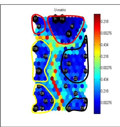
Figure 11(b) is U-Matrix visualization. The U-Matrix is visualized by three EMG features, RMS, MAV and STD. U-Matrix shows the predefined ‘T’ had been clustered by the EMG features. The predefined ‘T’ is scattered and hardly to obtain the class of angle movements. In Figure 11(b) six clustered data in red, yellow and black outline colour. The red line colour is defined as movements by angle of 60˚. It is because the small and large red outline colour is separated by small deviation(light blue colour). The yellow outline colour had about identical area of clustered data, it shows that the clustered data essentially of two type of difference data. The yellow outline clustered data is predicted as movements by angle of 120˚. While the black outline prediction goes to movements by angle of 90˚.

(8)

Figure 11(a): The Components Planes Of EMG Signals Features.

Figure 11(b): Visualization Of U-Matrix For 100 Neurons.

100 numbers of neurons is not sufficient amount to classify the movements. The test of increment number of neurons is carried until the data can be classified. The neurons are increased gradually by 10. The resulted of the test including the training time, quantization error and topographic error is compiled in Table 3. The number of neurons is updated in purpose to have the best matching unit of neighbourhood. The best matching unit function as tracking the node that produces the smallest distance. The

node requires smaller distance to pull the neighbouring nodes closer to the input vector.

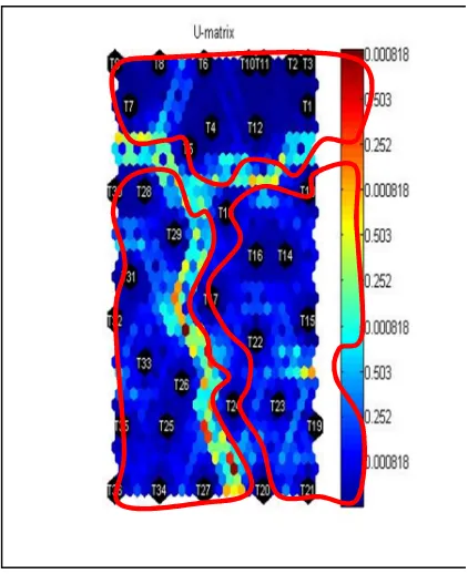
The result in Table 3 is gathered by training the neurons via MATLAB using SOM-Toolbox. The neurons training outcome the error and the training time for each increment of neurons. The errors values facilitate to decide the best number of neurons to classify the EMG signals for each movement. Neural Network is recognized by the winner in the neurons. In this experiment, the neurons win at number of 300. 300 neurons amount, resulted none topographic error and the smallest quantization error among the neurons. The training time in this experiment just reached 2 seconds. It is still categorized as rapid learning and applicable for features classification. The 300 neurons are closer to the input vector compared to the 100 neurons.

(9)

Figure 12(a): The Clustered Features Of EMG Signal In 300 Amount Of Neurons.

Figure 12(b): The Visualization Of Classified Angle Movements.

Figure 13: The Features Extraction In The Range Of Angle(Degree).

(10)

REFERENCES

[1]M. Z. Jamal, "Signal Acquisition Using Surface EMG and Circuit Design Considerations for Robotic Prosthesis," in Computational Intelligence in Electromyography Analysis –A Perspective on Current Applications and Future Challenges, InTech, 2012, pp. 427-448.

[2]P. M. S. K. Mr. Santosh S. Patil, "Feature Extraction of MES (MyoElectricSignal) using Temporal approach for prosthetic arm control," International Journal of Electronics and Computer Science Engineering.

[3]O. K. Pavel Stefanoviˇc, "Visual analysis of self-organizing maps," Nonlinear Analysis: Modelling and Control, vol. 16, no. 4, pp. 488-504, 2011.

[4]T. Kohonen, "Self-Organizing Formation of Topologically Correct Feature Maps," Biological Cybernetics, vol. 43, pp. 59-69, 1982.

[5]J. H. E. A. a. J. P. Juha Vesanto, "Self-Organizing Map in Matlab: the SOM Toolbox," Proceedings of the Matlab DSP COnference, vol. November 1999, pp. 35-40, 1999.

[6]M. H. Jali, M. F. Sulaima, T. A. Izzuddin, W. M. Bukhari, M. F. Baharom.: Comparative Study of EMG based Joint Torque Estimation AN ANN Models for Arm Rehabilitation Device.International Journal of Applied Engineering Research (IJAER), vol. 9, Number 10 (2014) pp. 1289-1301.

[7]M.H.Jali, T.A.Izzuddin, Z.H.Bohari, H.Sarkawi, M.F.Sulaima, M.F.Baharom, W.M.Bukhari, ”Joint Torque Estimation Model of sEMG Signal for Arm Rehabilitation Device Using Artificial Neural Network Techniques”,International Conference on Communication and Computer Engineering (ICoCoe), 2014.

[8]M.H.Jali, ‘Iffah Masturah Ibrahim, Mohamad FaniSulaima, WM Bukhari, Tarmizi Ahmad Izzuddin and Mohamad Na’im Nasir, “Features Extraction of EMG Signal using Time Domain Analysis for Arm

Rehabilitation Device”, International Conference on Mathematics on Mathematics, Engineering and Industrial Applications (ICoMEIA), 2014.

[9] M.H.Jali, T.A.Izzuddin, Z.H.Bohari, M.F.Sulaima, H.Sarkawi, “Predicting EMG Based Elbow Joint Torque Model Using Multiple Input ANN Neurons for Arm Rehabilitation “,UKSim-AMSS 16th International Conference on Modelling and Simulation, 2014

[10] M.H.Jali, Z.H.Bohari, M.F.Sulaima, M.N.M.Nasir and H.I.Jaafar, “Classification of EMG Signal Based on Human Percentile using SOM”, Research Journal of Applied Sciences, Engineering and Technology (RJASET), 2014.

(11)

Table 1: The Features Of Angle Movement.

Angle MAV RMS STD ZCS VAR

S1

60˚

0.001903 0.001981 0.001329 ₅₀ _1.68E-06

1.61E-03 0.001777 0.001329

48 1.99E-06

1.42E-03 1.75E-03 0.001325 ₄₄ _0.001325

90˚

0.00232 0.0027 0.0022 ₅₈ _2.66E-06

0.00231 0.00267 0.00219 ₄₃ _2.15E-06

0.00228 0.00254 0.00215 ₃₇ _2.189E-06

120˚

0.00318 0.00363 0.00311 ₃₉ _3.13E-06

0.00317 0.00365 0.0031 ₄₁ _2.71E-06

0.00317 0.00339 3.16E-03 ₅₁ _3.71E-06

S2

60˚

0.00174 0.00219 1.42E-03 ₆₅ _9.50E-07

0.00165 0.00189 1.38E-03 ₆₅ _9.75E-06

0.00164 0.00188 1.21E-03 ₃₁ _1.76E-06

90˚

0.00244 0.00286 0.00238

81 2.35E-06

0.00237 0.00285 0.00231 ₈₅ _2.62E-06

0.00232 0.00277 0.00228 ₅₄ _1.62E-06

120˚

0.00315 3.99E-03 0.00316 ₁₃ _3.56E-06

0.00316 3.98E-03 0.00318 ₃₃ _3.93E-06

0.00315 0.00384 0.00314 ₄₅ _3.42E-06

S3

60˚

9.75E-04 0.0019 0.00124 ₂₇ _8.34E-07

9.15E-04 0.00162 0.00133 ₁₉ _1.22E-06

9.13E-04 1.61E-03 1.10E-03

19 8.38E-07

90˚

0.002 0.00239 0.00209 ₂₃ _1.24E-06

0.00189 0.00231 0.00207 ₁₇ _1.93E-06

0.00186 0.00228 0.00205

41 1.75E-06

120˚

0.00282 0.00318 0.00314 ₃₁ _2.49E-06

0.00291 0.00316 0.00307 ₅₀ _2.53E-06

2.98E-03 0.00315 0.00302

23 2.60E-06

S4

60˚

0.00161 0.00198 0.00133 ₁₅ _1.89E-06

0.00154 0.00185 0.00129 ₁₉ _1.46E-06

0.00141 1.73E-03 0.00127

20 2.00E-06

90˚

0.00233 0.00246 2.44E-03 ₃₀ _2.21E-06

0.00231 0.00243 0.00237 ₂₅ _2.75E-06

2.23E-03 0.00242 0.0026

27 2.06E-06

120˚

0.0033 0.00391 0.00317 ₃₄ _3.05E-06

0.0032 0.00382 0.00313 ₃₆ _3.16E-06

(12)

Table 2: Predefine T For Unsupervised Learning.

T DESCRIPTION SUBJECT

T1, T2, T3 Movements by angle of 60˚

S1

S2

S3

S4

(13)

Table 3: The Training Data Result.

No. of Neuron

Training Time

Quantization Error

Topographic Error

100 0s 0.026 0.056

110 0s 0.025 0.028

120 0s 0.023 0.028

130 0s 0.022 0.000

140 0s 0.018 0.028

150 1s 0.014 0.028

160 1s 0.015 0.000

170 1s 0.015 0.028

180 1s 0.016 0.028

190 1s 0.013 0.028

200 1s 0.011 0.000

210 1s 0.009 0.000

220 1s 0.009 0.000

230 1s 0.006 0.028

240 1s 0.007 0.000

250 2s 0.007 0.000

260 2s 0.006 0.000

270 2s 0.004 0.000

280 2s 0.004 0.000

290 2s 0.003 0.000