The Immunization Performance
of Traditional and Stochastic Durations:
A Mean-Variance Analysis
∗ Pascal François†HEC Montréal Université de Rennes 1 and CNRSFranck Moraux July 30, 2008
∗We thank Nihat Aktas, Luc Bauwens, Simon Lalancette, Nicolas Papageorgiou and Isabelle Platten,
as well as seminar participants at the Luxembourg School of Finance, the University of Paris XII, and the UCL (CORE/LSM joint seminar) for helpful comments. François acknowledges financial support from IFM2 and FQRSC. Moraux acknowledges financial support from IAE Rennes and CREM (CNRS 6211).
The usual disclaimer applies.
†Corresponding author. Postal address: HEC Montréal, Department of Finance, 3000
T I P T S D : A M -V A
Abstract: This paper provides a mean-variance analysis of immunization strategies
that trade off coupon reinvestment risk with resale price risk. For static immunization strategies, neither traditional nor stochastic durations fall in the set of efficient horizons that we characterize explicitly. This finding is robust across various interest rate environ-ments and bond characteristics. It can explain the poor immunization results obtained by the comparative study of Gultekin and Rogalski (1984) on durations. When dynamic port-folio rebalancing is allowed, the ranking of performance remains the sames, but spreads between traditional and stochastic durations dramatically narrow. We therefore obtain that immunization performance is more driven by strategy sophistication rather than by the choice of duration, which corroborates the empirical finding of Agca (2005). Our re-sults are robust under the two-factor term structure model with stochastic volatility of Longstaff and Schwartz (1992).
1 Introduction
Immunizing bond portfolios against interest rate fluctuations is a major challenge in fixed-income management. Since the work of Macaulay, duration has been viewed as a relevant tool for immunization purposes. Yet, extending the definition of duration to account for stochastic interest rates is a non trivial exercise. Several papers propose new definitions of stochastic duration: Cox, Ingersoll and Ross (1979) and Wu (2000) for equilibrium single factor models, Au and Thurston (1995) and Frühwirth (2002) for Heath-Jarrow-Morton models, and Munk (1999) for multi-factor models. Despite these theoretical contributions, empirical studies on immunization performance do not conclude on the superiority of stochastic durations over traditional ones. Gultekin and Rogalski (1984) find that all of the seven durations they study induce disappointing results. Studies edited by Kaufman, Bierwag and Toevs (1983) as well as the more recent works of Wu (2000) and Agca (2005) reach similar conclusions. All this statistical evidence calls for investigating the immunization performance that one can expect from traditional and stochastic durations. By contrast to earlier work that measures immunization performance ex post using
bond data over a sample period, our paper is, to the best of our knowledge, the first at-tempt at measuring immunization performanceex ante by analyzing immunization
strat-egy returns within the mean-variance framework. Specifically, we examine a couple of stylized immunization strategies. The basic strategy captures the fundamental issue in duration-based immunization, that is, trading off coupon reinvestment risk and resale price risk (see e.g. Sundaresan, 2002). The other strategy is a dynamic extension that allows for frequent rebalancing.
du-ration that achieves the lowest variance in returns (and call it the minimum variance duration). We obtain that neither traditional nor stochastic durations fall in the set of efficient horizons. This result is robust across various interest rate parameters and bond characteristics. This finding sheds a new light on prior evidence: The ex ante inefficiency of both traditional and stochastic duration-based strategies could explain the poor immu-nization results obtained by Gultekin and Rogalski (1984) in their comparative study of ex post performance.
Next, we examine a dynamic immunization strategy which allows for monthly rebal-ancing to keep matching the coupon reinvestment horizon with the duration according to the path followed by the spot rate. Monte Carlo simulations show that differences in immunization performance across durations are narrowed. This finding confirms the empirical work of Agca (2005) who concludes that immunization performance is more driven by strategy sophistication rather than by the choice of duration. Yet, the same performance ranking across durations holds: While all strategies exhibit the same target expected return, the ones using stochastic duration generate the most volatile returns, followed by the ones using traditional durations. Using the test recently developed by Opdyke (2007), we cannot reject at any standard level of confidence the superiority of Sharpe ratios of immunization strategies based on the minimum variance duration.
To check the extent to which our results could be driven by the choice of term structure model, we repeat the analysis under the two-factor term structure model with stochastic volatility of Longstaff and Schwartz (1992). Monte Carlo results are robust to this alternate specification.
The analysis is conducted under two different term structure models. We conclude in section 6.
2 Term structure model and durations
The mean-variance analysis is carried out under the Vasicek (1977) term structure model. This setting allows for explicitly characterizing the mean and the variance of strategy returns.1 The term structure is driven by the instantaneous risk-free ratertwhich follows
a Gaussian mean-reverting process under the risk-neutral measure
drt= α (β + λ − rt) dt + ηdZt. (1)
In equation (1), the (physical) process {rt}t≥0 reverts to the long-term mean β,α is the
reversion speed, λ is the market price of risk, and random increments are driven by the
Brownian motionZtwith volatilityη. The time−tvalue of the default-free discount bond
with principal $1 and time to maturity τ, denoted byP (t, τ), is given by P (t, τ) = a (τ) exp (−b (τ) rt) ,
with
a (τ) = exp (b (τ) − τ)
α2(β + λ) − η2/2
α2 −η
2b2(τ) 4α
b (τ) = 1 − exp (−ατ)α .
Let Pc(t, T − t)denote the time−tvalue of the coupon bond. Without loss of generality,
we assume a continuous coupon stream c so that Pc(t, T − t) = c
T
t P (t, k − t) dk + P (t, T − t) .
One denotes by Ω = {r0, α, β, λ, η} the set of parameters. Typical shapes of the
zero-coupon yield curves generated by the Vasicek model are: increasing, decreasing and humped. We work under three sets of parameters to capture different interest rate en-vironments. Figure 1 details the parameterizations and shows the corresponding term structures.
We consider three different duration measures: the Macaulay and the Fisher-Weil du-rations among the so-called “traditional” measures, and the Cox-Ingersoll-Ross stochastic duration. For a coupon bond with face value 1 and continuous coupon c, the Macaulay
duration is defined by
θmac = c 0Tke−ykdk + Te−yT Pc(0, T) ,
where y is the continuously compounded yield-to-maturity on the coupon bondPc(0, T).
The Fisher-Weil duration is
θfw = c 0T kP (0, k) dk + TP (0, T)
Pc(0, T) .
These two traditional durations are widely used in the industry. On a theoretical ground, Ingersoll, Skelton and Weil (1978) show that these durations are valid risk measures when changes in the term structure are limited to parallel shifts. Cox, Ingersoll and Ross (1979) propose to define the stochastic duration as the maturity, expressed in units of time, of a discount bond with same basis risk as the initial instrument. Therefore, in the context of the Vasicek model2
θsto= b−1 c T
0 b (k) P (0, k) dk + b (T) P (0, T) Pc(0, T)
where
b−1(u) = −α1 ln(1 − αu) , u < α1.
2It is well known that the extended Vasicek model is equivalent to the one-factor Heath-Jarrow-Morton model with exponentially decaying volatility. Consequently, the duration
θsto of this paper is analogous to the measure used by Au and Thurston (1995) example
3 The basic immunization strategy
We introduce a stylized strategy that captures the trade-off between coupon reinvestment risk and resale price risk. Consider an investor who is currently long in one coupon bond with face value 1, maturityT and continuous couponc. The strategy with horizonθ (0 ≤ θ ≤ T)consists in (i) holding the coupon bond between dates0andθ, (ii) re-investing
each time−tcoupon in the discount bondP (t, θ − t), and (iii) closing the positions at time θ.3
The value πθ of the investor’s portfolio at dateθ is πθ = Pc(θ, T − θ) + c
θ 0
ds
P (s, θ − s). (2)
Settingθ = 0, the strategy reduces to the instantaneous resale of the coupon bond. Setting θ = T, the strategy reduces to the buy and hold of the coupon bond. As the investor
selects a longer θ, his or her portfolio gets more exposed to coupon reinvestment risk and
less exposed to resale price risk. The immunization strategy looks for the best trade-off.
Proposition 1 For any horizon θ, the random value of the basic immunization strategy
has mean and variance respectively equal to
E (πθ) = c T
θ A(θ, k, −) dk + A (θ, T, −) + c θ
0 A (s, θ, +) ds. and
var (πθ) = Σ2P + Σ2C+ 2ΣP C
where
Σ2
P = 2c2 T θ
T
j A (θ, k, −) A (θ, j, −) B (t, u, v, ±) B (θ, k, θ, j, +) dkdj +A(θ, T, −)2B (θ, T, θ, T, +)
+2c T
θ A (θ, k, −) A (θ, T, −) B (θ, k, θ, T, +) dk, Σ2
C = 2c2 θ 0
θ
s A (s, θ, +) A(u, θ, +) B (s, θ, u, θ, +) dsdu, ΣP C = c2
T θ
θ
0 A(θ, k, −) A(s, θ, +) B (s, θ, θ, k, −) dsdk
+c θ
0 A(θ, T, −) A (s, θ, +) B (s, θ, θ, T, −) ds, with
A (t, u, ±) = a (u − t)−(±1)exp ±
b
(u
−t
)m
t+12b
2(u
−t
)v
tB
(t,u,v,w,
±) = exp (±b
(u
−t
)b
(w
−v
)g
t,v) − 1and
m
t : =E
(r
t) =r
0e
−αt+β
1 − e−αt, vt : = var (rt) = η2
2α 1 − e−2αt ,
gt,u : = cov (rt, ru) = η2exp (−α (t + u))exp (2αt) − 1
2α .
Proof: see appendix.
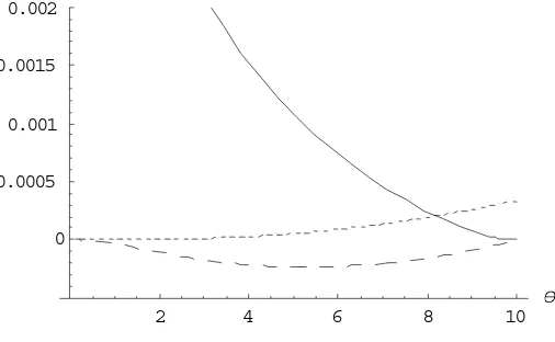
Proposition 1 allows for a variance decomposition of the basic immunization strategy returns.4 The variances corresponding to resale price risk and coupon reinvestment risk
involve Σ2
P and Σ2C, respectively. The immunization strategy also induces a covariance
term involving ΣP C. In line with intuition, Figure 2 shows that the basic immunization
strategy with a longer horizon decreases the exposure to resale price risk and increases 4Without loss of generality, the analysis will focus on annualized returns defined by
the risk of coupon reinvestment. The covariance component typically reduces the total risk and its effect is the strongest around half time to maturity. Similar patterns (not reported) hold for different interest rate environments.
Proposition 2 For the instantaneous resale strategy, the return has mean and standard
deviation
limE(Rθ)
θ→0+ = r
limσ(Rθ)
θ→0+ = η · b θ
sto .
Proof: see appendix.
At the limit, buying and immediately selling the coupon bond yields a return equal to the instantaneous spot rate. The volatility of this strategy is that of the instan-taneous spot rate multiplied by the sensitivity of the coupon bond (since bθsto = P′
c(t, T − t) /Pc(t, T − t)).
4 Mean-variance analysis
In this section, we characterize the set of efficient basic immunization strategies. Then we assess the performance of basic immunization strategies using the duration measures introduced in section 2.
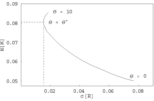
Figure 3 plots, for every horizonθ, the returns of the basic immunization strategy in
the mean-standard deviation space(0, σ (Rθ) , E (Rθ)). Inspection of Figure 3 shows that
there exists a minimum variance horizon θ∗. This is the horizon that achieves the lowest
variance trade-off between coupon reinvestment risk and resale price risk. The same plot is represented in Figure 4 for the other interest rate environmentsΩ2 (decreasing yield curve)
andΩ3 (humped yield curve), as well as in Figure 5 for different bond characteristics. The
and the most “north-western” returns are obtained with θ ranging from θ∗ toT. In the
absence of coupons,θ∗ = T. Henceθ∗can be interpreted as a duration. For the remainder
of the paper, it will be referred to as the minimum variance duration.5
Proposition 3 The basic immunization strategy with horizonθis mean-variance efficient
if and only if
θ ≥ θ∗ =argmin
θ [σ(Rθ)].
Corollary The buy and hold strategy (θ=T) is mean-variance efficient.
Using Propositions 1 and 3, we can gauge the performance of immunization strategies
based on traditional and stochastic durations. Results are displayed in Figure 6 using the base case parameters of Figure 3. As a robustness check, Tables 1, 2 and 3 show the means and standard deviations of returns for different interest rate environments (Table 1), and different coupon rates and maturities (Tables 2 and 3). Sharpe ratios are also reported.6
Our findings can be summarized in three main points.
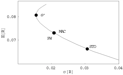
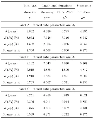
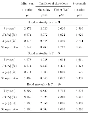
First, both traditional and stochastic durations are always below the minimum variance duration, and therefore induce inefficient immunization strategies. Oddly enough, all these durations induce an underexposure to the coupon reinvestment risk. Second, The Cox-Ingersoll-Ross duration is systematically the lowest among the three measures. Hence immunization strategies based on traditional durations outperform those based on the stochastic duration, especially for long bonds. This finding helps explain why previous empirical studies fail to prove the superiority of stochastic durations for immunization purposes. Third, the strategy based on Macaulay duration and that based on Fisher-Weil duration yield very similar immunization results.
5Note that, just like traditional and stochastic durations, the minimum variance dura-tion need not be a strictly increasing funcdura-tion of maturity.
5 Dynamic immunization strategies
In this section, we consider a dynamic extension of the basic immunization strategy. Specif-ically, the coupon reinvestment horizon is not determined once at initial date, but rather recalculated periodically. As the spot rate changes over time, all the accumulated coupons that were previously invested at datetin the zero coupon bond with maturityθtare then
reinvested in the zero coupon bond with maturity θt+∆t.7
As in the former section, we use the traditional and stochastic durations to determine the reinvestment horizons {θt}t≥0. We then challenge these strategies with the one
con-sisting in minimizing the variance of the investment strategy returns (this minimization is now performed periodically).
5.1 Strategy description
We discretize the time interval[0, T]and we denote by∆tthe (arbitrarily small) time step.
This time step represents the investor’s rebalancing frequency. The dynamic immunization strategy is described as follows.
1. Buy the coupon bond with maturityT at time 0,
2. At any datei∆t, the accumulated capitalized coupons (acci) are defined as acci =
i
k=1 c∆t
⎛ ⎝i
j=k
Pj∆t, θ(j−1)− j∆t P (j − 1) ∆t, θ(j−1)− (j − 1) ∆t
⎞ ⎠ ,
and they will be invested in the zero coupon bond with maturity θ(i),
3. At the same date, the next reinvestment horizonθ(i) is calculated along the chosen
duration measure (see the appendix for details),
4. Accumulated capitalized coupons are reinvested until dateΘ = I∆t where I = inf i ≥ 0 : θ(i)< ∆t .
Note that the starting point of the dynamic strategy coincides with the basic immu-nization strategy defined in the above section. That is, we have thatπ0,θ = πθ and hence θx
(0)= θx, wherexcharacterizes the duration measure. Then basic and dynamic strategies
differ as the spot rate follows a particular path and the investor updates the reinvestment horizon accordingly.
5.2 Monte Carlo results
We carry out a mean-variance analysis of dynamic strategies by simulating a large number of scenarios. Without any loss in generality, we assume the investor’s rebalancing frequency to be monthly (∆t = 1/12). The Vasicek process for the spot rate is simulated using the
Euler scheme. To reduce the bias caused by time discretization, the Euler scheme uses a daily time step(∆t = 1/360). Then the monthly interest rate process is simply obtained
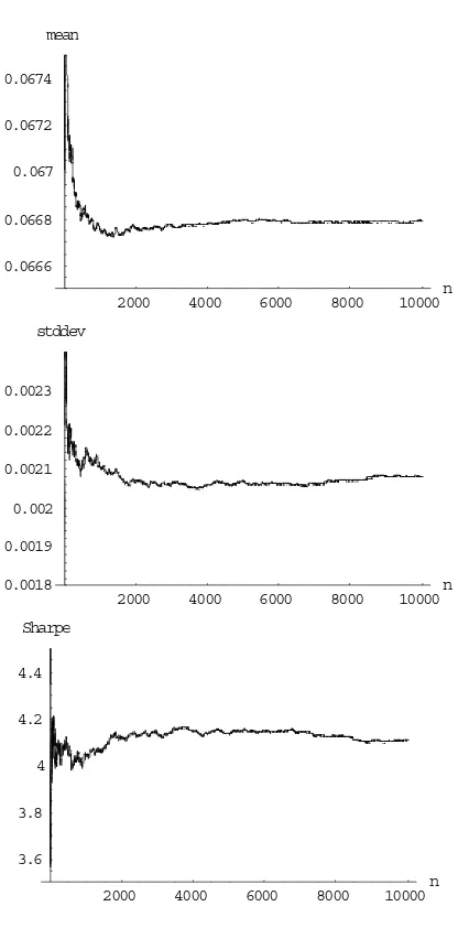
by taking one every thirty realizations. The same set of sample paths is used to run all dynamic strategies. The number of sample paths is set to 10,000. Figure 7 shows the convergence of the Monte Carlo experiment for the mean and standard deviation of returns as well as for the Sharpe ratio. It can be seen that the number of sample paths warrants a sufficient level of accuracy for the numbers reported in our tables.
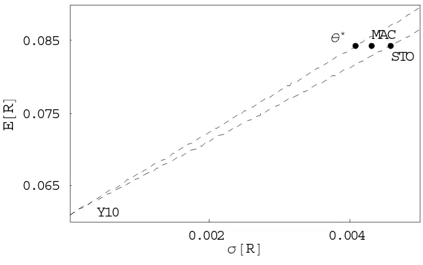
Figure 8 and Table 4 report the mean-variance analysis. Not surprisingly, Sharpe ratios are higher than in the basic case (Table 3), especially for long maturities, because of the value created by updating information.
immunization performance is more driven by strategy sophistication rather than by the choice of duration. The empirical study of Agca (2005) reaches a similar conclusion.
Yet, we observe that the performance ranking across durations seems to remain the same — the strategy based on the stochastic duration exhibiting the poorest performance. However, because values in Table 4 are Monte Carlo estimates, they suffer from some degree of uncertainty so that such a conclusion should be cautioned. Actually, we have used the one-tailed test exposed in Opdyke (2007) to test whether Sharpe ratios obtained with traditional and stochastic durations are significantly lower than those implied by the minimum variance strategy (given that every Sharpe ratio has its own confidence interval).8 In all pairwise comparisons the superiority of Sharpe ratios of strategies using
the minimum variance duration could not be rejected at any standard level of confidence. This means that, although dynamic rebalancing aligns performance of strategies, the same ranking across durations holds statistically.
5.3 Alternative interest rate model
We check the extent to which our results could be driven by the chosen interest rate model. Simulations of the dynamic immunization strategies are performed under a different inter-est rate model. Specifically, we choose to work under the Longstaff and Schwartz (1992) two factor model where
drt = αγ + βη −βδ − αξ β − α rt−
ξ − δ β − αVt
dt
+α
βrt− Vt
α (β − α)dWt1+ β
Vt− αrt β (β − α)dWt2
and
dVt = α2γ + β2η −αβ (δ − ξ)β − α rt−βξ − αδβ − α Vt dt
+α2
βrt− Vt
α (β − α)dWt1+ β2
Vt− αrt β (β − α)dWt2,
where W1 and W2 are two independent Brownian motions and α, β, γ, δ, η and ξ are
positive constant parameters.
Simulating the strategy described in subsection 5.1 requires (i) knowledge of the dis-count bond value function and (ii) determination of the coupon reinvestment horizon. The Longstaff and Schwartz (1992) model allows for a closed-form solution toP (t, τ). As
for durations, Macaulay and Fisher-Weil measures keep the same definitions. Moreover, Munk (1999) solves for the stochastic (Cox-Ingersoll-Ross type) duration in the Longstaff and Schwartz (1992) model. He finds thatθsto is the solution to
0 = α (βr − V )ϕ2 eϕθsto− 1 2am θsto 2− Ka2
+β (V − αr) ψ2
eψθsto− 1 2bm θsto 2− K2
b
,
with ϕ = 2α + δ2,ψ =2β + (ξ + λ)2,λis the market price of risk, and
am(x) = 2ϕ
(δ + ϕ) (eϕx− 1) + 2ϕ bm(x) = (ξ + λ + ψ) (e2ψψx− 1) + 2ψ
Ka = c tT P (t, k − t) eP ϕ(k−t)− 1 am(k − t) dk
c(t, T − t)
+P (t, T − t) eϕ(T−t)− 1 am(T − t) Pc(t, T − t)
Kb = c tT P (t, k − t) eψ(k−t)− 1 bm(k − t) dk Pc(t, T − t)
+P (t, T − t) ePψ(T−t)− 1 bm(T − t)
c(t, T − t) .
thirty realizations of the process to work with monthly values. When simulating processes with stochastic volatility, the standard Euler scheme can generate negative variance with non-zero probability, which causes the time stepping scheme to fail. To avoid this problem, we rely on the so-called full truncation scheme as described in Lord et al. (2006).9
Parameter values are set very close to the ones obtained by Jensen (2001) who estimates the Longstaff-Schwartz model on the weekly US 3-month T-Bill over the 1954 — 1998 period. Specifically, we take α = 0.0003, β = 0.015, γ = 40,δ = 0.25, ξ = 4 andη = 5.
Setting the initial values of r = 0.05 and V = 0.0002, we obtain an increasing term
structure similar to the one generated by interest rate environmentΩ1.
As shown in Table 5, results are very similar to the Vasicek case. Differences in Sharpe ratios across durations are narrowed. We also apply Opdyke (2007) tests to take uncertainty around Monte Carlo estimates into account. Again, we find that the same ranking across Sharpe ratios statistically prevails: While we cannot reject equal Sharpe ratios for the strategies using the Macaulay and the Fisher-Weil durations, the strategy using the stochastic duration displays a significantly lower Sharpe ratio at any standard level of confidence. Our previous findings are therefore robust to the choice of the term structure model.
6 Concluding remarks
narrowed. The analysis is conducted under a Gaussian interest rate model, which allows for analytical solutions for the mean and the variance of strategies and for an explicit characterization of the mean-variance efficient set. Yet, the same performance ranking across duration measures holds under an alternative two-factor term structure model with stochastic volatility. Our results support past empirical studies by concluding that tradi-tional durations can outperform stochastic duration for immunization purposes and that strategy sophistication matters more than the choice of duration. In addition, by showing that both traditional and stochastic durations may not fall in the set of efficient horizons, our work offers an explanation as to why previous empirical studies on immunization find disappointing performance for all duration-based strategies.
Actually, the imperfect adequacy of duration for immunization purposes may find its origins from the ambivalent definition of duration. Most available durations, especially the stochastic one, are defined as the bond price elasticity with respect to the relevant risk factor(s). These measures are essentially Hicks-type durations built for hedging purposes.
Alternatively, duration can be defined as the holding period over which the portfolio made of all reinvested coupons plus the present value of the bond is immune to interest rate changes. This is theMacaulay-type duration, which justifies its use in immunization
strategies. Unfortunately, it is well known that the hedging and immunization definitions coincide only when the term structure is flat and subsequently undergoes parallel shifts. Ourex ante mean-variance analysis and previousex post empirical studies both emphasize
the limitations in implementing an immunization strategy with a duration defined in a hedging sense.
References
[1] Agca, S., 2005, The performance of alternative interest rate risk measures and im-munization strategies under a Heath-Jarrow-Morton framework, Journal of Financial and Quantitative Analysis 40, 645—669.
[2] Andersen, L., 2008, Simple and efficient simulation of the Heston stochastic volatility model, Journal of Computational Finance 11, 1—42.
[3] Au, K. and D. Thurston, 1995, A new class of duration measures, Economic Letters 47, 371—375.
[4] Cox, J., J. Ingersoll and S. Ross, 1979, Duration and the measurement of basis risk, Journal of Business 52, 51—61.
[5] Frühwirth, M., 2002, The Heath Jarrow Morton duration and convexity: A general-ized approach, International Journal of Theoretical and Applied Finance 5, 695—700. [6] Gultekin, B. and R. Rogalski, 1984, Alternative duration specifications and the
mea-surement of basis risk: Empirical tests, Journal of Business 57, 241—264.
[7] Ingersoll, J., J. Skelton and R. Weil, 1978, Duration forty years later, Journal of Financial and Quantitative Analysis 13, 627—650.
[8] Jensen, M. B., 2001, Efficient method of moments estimation of the Longstaff and Schwartz interest rate model, Working paper, Aarhus University.
[9] Kaufman, G., G. Bierwag and A. Toevs, 1983, Innovation in bond portfolio manage-ment: Duration analysis and immunization, JAI Press.
[11] Longstaff, F. and E. Schwartz, 1992, Interest rate volatility and the term structure: A two-factor general equilibrium model,Journal of Finance 47, 1259—1282.
[12] Lord, R., R. Koekkoek and D. van Dijk, 2006, A comparison of biased simulation schemes for stochastic volatility models, Tinbergen Institute discussion paper TI 2006-046.
[13] Munk, C., 1999, Stochastic duration and fast coupon bond option pricing in multi-factor models,Review of Derivatives Research 3, 157—181.
[14] Opdyke, J.D., 2007, Comparing Sharpe ratios: So where are the p−values?, Journal
of Asset Management 8, 308—336.
[15] Sundaresan, S., 2002, Fixed income markets and their derivatives, South Western. [16] Vasicek, O., 1977, An equilibrium characterization of the term structure, Journal of
Financial Economics 5, 177—188.
Appendix
Proof of Proposition 1
The mean of the value process is given by
E (πθ) = c T
θ E (P (θ, k − θ)) dk + E (P (θ, T − θ)) + c θ 0 E
1 P (s, θ − s)
ds.
For any given
t
andτ
, we have thatE
(P
(t,τ
)) =a
(τ
)E
(exp(−b
(τ
)r
t)).
Since
r
t is Gaussian with meanm
t:=E
(r
t) =r
0e
−αt+ β 1 − e−αtand variance
vt:= var (rt) = η 2
2α 1 − e−2αt , we obtain
E
(P
(t,τ
)) =a
(τ
) exp −b
(τ
)m
t+12b
2(τ
)v
t.
Similarly,
E
P
(1t,τ
) =a
1 (τ
)exp
b
(τ
)m
t+12
b
2(τ
)v
t.
Hence
E
(π
θ) =c
Tθ
a
(k
− θ) exp −b
(k
−θ
)m
θ+ 12
b
2(k
−θ
)v
θdk
+a
(T
−θ
) exp
−
b
(T
−θ
)m
θ+ 12b
2(T
−θ
)v
θ+
c
θ 01
a
(θ
−s
)expb
(θ
−s
)m
s+ 1As for variance, we have that
var (πθ) = c2var T
θ P (θ, k − θ) dk + var (P (θ, T − θ)) +2c · cov T
θ P (θ, k − θ) dk, P (θ, T − θ) +c2var θ
0
1
P (s, θ − s)ds
+2c2cov
T
θ P (θ, k − θ) dk, θ
0
1
P (s, θ − s)ds +2c · cov
P (θ, T − θ) , θ 0
1
P (s, θ − s)ds .
Which yields, for k ≥ j and u ≥ s
var (πθ) = 2c2 T θ dj
T
j cov (B (θ, k − θ) , B (θ, j − θ)) dk +var (B (θ, T − θ))
+2c T
θ cov (B (θ, k − θ) , B (θ, T − θ)) dk +2c2 θ
0 ds θ s cov
1
B (u, θ − u),B (s, θ − s)1
du
+2c2 θ 0 ds
T
θ cov B (θ, k − θ) , 1 B (s, θ − s)
dk
+2c θ
0 cov B (θ, T − θ) , 1 B (s, θ − s)
ds.
First, we compute var (P (t, τ)) for any givent andτ. We have that var (P (t, τ)) = a2(τ) var (exp (−b (τ) r
t)) .
Since exp (−b (τ) rt) is log-normal, we get var (P (t, τ)) = a2(τ) exp −2b (
τ
)m
t+
b
2(τ
)v
t expb
2(τ
)v
t − 1.
Similarly,
var
P
(1t,τ
) =a
21 (τ
)exp
Next, we compute
cov
(P
(t,τ
),P
(t,ζ
))for any givent
,τ
andζ
. We have thatcov
(P
(t,τ
),P
(t,ζ
)) =a
(τ
)a
(ζ
)cov
(exp(−b
(τ
)r
t),
exp(−b
(ζ
)r
t)).
Note that the last covariance can also be written as
E
(exp (− (b
(τ
) +b
(ζ
))r
t)) −E
(exp (−b
(τ
)r
t))E
(exp(−b
(ζ
)r
t)),
which yields
cov
(P
(t,τ
),P
(t,ζ
)) =a
(τ
)a
(ζ
) exp
− (
b
(τ
) +b
(ζ
))m
t+21((b
(τ
) +b
(ζ
)))2v
t−
a
(τ
)a
(ζ
)exp
− (
b
(τ
) +b
(ζ
))m
t+12b
2(τ
)v
t+12b
2(ζ
)v
t=
a
(τ
)a
(ζ
) exp− (
b
(τ
) +b
(ζ
))m
t+12
b
2(τ
)v
t+ 12
b
2(ζ
)v
t ×[exp (b
(τ
)b
(ζ
)v
t) − 1].
Now we compute cov 1
P (s,τ),P (u,ζ)1
for any givens,u ≥ s,τ andζ. We have that cov
1
P
(s,τ
),
P
(u,ζ
1 ) =a
(τ
)1a
(ζ
)cov
(exp (b
(τ
)r
s),
exp (b
(ζ
)r
u)).
Note that the last covariance can also be written asE
(exp (b
(τ
)r
s+b
(ζ
)r
u)) −E
(exp(b
(τ
)r
s))E
(exp(b
(ζ
)r
u)),
or, equivalently
exp
b
(τ
)m
s+b
(ζ
)m
u+1 2b
2(
τ
)v
s+b
2(ζ
)v
u+ 2b
(τ
)b
(ζ
)g
s,u− exp
b
(τ
)m
s+12b
2(τ
)v
sexp
b
(ζ
)m
u+12b
2(ζ
)v
u,
with
gs,u:= cov (rs, ru) = η2exp (−α (s + u))exp (2αs) − 1
Hence
cov
P
1 (s,τ
),
1
P
(u,ζ
) =a
(τ
)1a
(ζ
)exp
b
(τ
)m
s+b
(ζ
)m
u+1 2b
2(
τ
)v
s+b
2(ζ
)v
u+ 2b
(τ
)b
(ζ
)g
s,u−
a
(τ
)1a
(ζ
)expb
(τ
)m
s+21b
2(τ
)v
s expb
(ζ
)m
u+ 21b
2(ζ
)v
u.
cov
P
(1s,τ
),
P
(u,ζ
1 )=
a
(τ
)1a
(ζ
)expb
(τ
)m
s+b
(ζ
)m
u+ 12b
2(τ
)v
s+12b
2(ζ
)v
u [exp (b
(τ
)b
(ζ
)g
s,u) − 1].
Finally, the computation of cov P (θ, τ) , 1 P (u,ζ)
for any given θ,θ ≥
u
,τ
andζ
yieldscov P
(θ,τ
),
P
1 (u,ζ
) =a
a
((τ
ζ
))exp
−
b
(τ
)m
θ+b
(ζ
)m
u+12b
2(τ) vθ+12b2(ζ) vu[exp (−b (τ) b (ζ) gu,θ) − 1] .
Combining all these results completes the proof.
Proof of Proposition 2
Applying Itô’s lemma,
dPc(t, T − t) = ∂Pc(t, T − t)
∂t dt +∂P
c(t, T − t)
∂r dr +12∂
2Pc(t, T − t)
∂r2 (dr)2. (3) Note that
∂Pc(t, T − t)
∂t = c
T t
∂P (t, k − t)
∂t dk − cP (t, 0) +∂P (t, T − t)∂t ∂Pc(t, T − t)
∂r = c
T t
∂P (t, k − t)
∂r dk +∂P (t, T − t)∂r ∂2Pc(t, T − t)
∂r2 = c
T ∂2P (t, k − t) ∂r2 dk +∂
2P (t, T − t)
Hence, equation (3) becomes
dPc(t, T − t) = c T t
∂P (t, k − t)
∂t dk − cP (t, 0) +∂P (t, T − t)∂t +α (β − rt) c
T t
∂P (t, k − t)
∂r dk + α (β − rt)
∂P (t, T − t) ∂r +η22c T
t
∂2P (t, k − t) ∂r2 dk + η
2 2 ∂
2P (t, T − t)
∂r2 dt
+η
c T t
∂P (t, k − t)
∂r dk +∂P (t, T − t)∂r dZt.
Terms indtcan be simplified as E (dPc(t, T)) = c
T t
∂P (t, k)
∂t + α (β − rt)∂P (t, k)∂r +η 2 2 ∂
2P (t, k)
∂r2 dk dt
−cdt + ∂P (t, T)∂t + α (β − rt)∂P (t, T)∂r +η 2 2 ∂
2P (t, T) ∂r2
dt.
In absence of arbitrage, we have, for any u > t
∂P (t, u − t)
∂t + α (β − rt)∂P (t, u − t)∂r +η 2 2 ∂
2P (t, u − t)
∂r2 = rtP (t, u − t) .
Hence
E (dPc(t, T − t) + cdt) = rtc T
t P (t, k − t) dk
dt + rtP (t, T − t) dt,
E
dPc(t, T − t) + cdt Pc(t, T − t)
= rtdt.
As for standard deviation, we obtain from equation (3)
σ
dPc(t, T − t) + cdt Pc(t, T − t)
= P η
c(t, T − t)
c T
t
∂P (t, k − t)
∂r dk +∂P (t, T − t)∂r
.
Hence, from the definition of θsto σ
dPc(t, T − t) + cdt Pc(t, T − t)
Dynamic strategy description
For the minimum variance duration, the next reinvestment horizon θ∗
(i) is calculated as
argmin
θ [σ(Ri,θ)] where the value process of the dynamic immunization strategy is given
by
πi,θ =Pc(θ, T − θ) +c θ i∆t
ds
P (s, θ − s) +P (i∆t, θ − i∆t)acci .
Note that the last term is known at date i∆t and therefore does not interfere in the
computation of vari(πi,θ).
Similarly, the next reinvestment horizonθ(i) for all other durations is calculated as θmac(i) = c
T
i∆t(k − i∆t) e−y(k−i∆t)dk + (T − i∆t) e−y(T −i∆t) c i∆tT e−y(k−i∆t)dk + e−y(T −i∆t) ,
where y is the continuously compounded yield-to-maturity on the coupon bond θfw(i) = c
T
i∆t(k − i∆t) P (i∆t, k − i∆t) dk + (T − i∆t) P (i∆t, T − i∆t) c i∆tT P (i∆t, k − i∆t) dk + P (i∆t, T − i∆t) ,
θsto
(i) = b−1 c T
i∆tb (k − i∆t) P (i∆t, k − i∆t) dk + b (T − i∆t) P (i∆t, T − i∆t) c i∆tT P (i∆t, k − i∆t) dk + P (i∆t, T − i∆t) ,
The annualized return of the dynamic immunization strategy is then given by
RΘ = Θ1 Pc(Θ, T) + accP Θ− Pc(0, T)
Figures
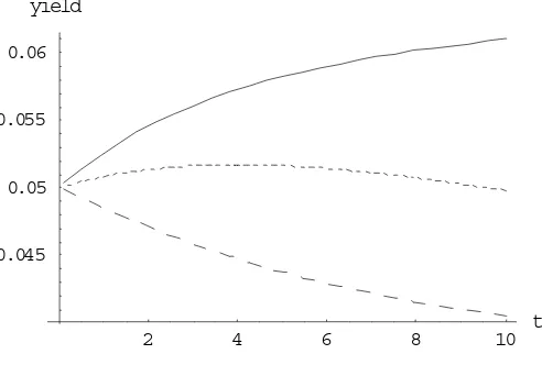
Figure 1: Sets of parameters and their implied zero-coupon yield curves.
The three sets of parameters are:
Set Shape r0 α β η
Ω1 Increasing 0.05 0.3 0.07 0.03 Ω2 Decreasing 0.05 0.3 0.04 0.03 Ω3 Humped 0.05 0.1 0.07 0.03
andλ = 0across the three sets.
2 4 6 8 10 t
0.045 0.05 0.055 0.06
yield
Figure 1 plots the zero-coupon yield curve corresponding to the set Ω1 (straight line), Ω2
Figure 2: Variance decomposition
of the basic immunization strategy returns.
2 4 6 8 10 θ
0 0.0005
0.001 0.0015 0.002
Figure 3: Basic immunization strategy returns
in the mean-standard deviation space.
0.02 0.04 0.06 0.08
σ@RD 0.05
0.06 0.07 0.08 0.09
E
@
R
D
θ = θ∗
θ = 10
θ = 0
Figure 3 plots the returns of the basic immunization strategy in the mean-standard deviation space for every horizonθ. Interest rate environment isΩ1. Bond maturity isT = 10, coupon rate
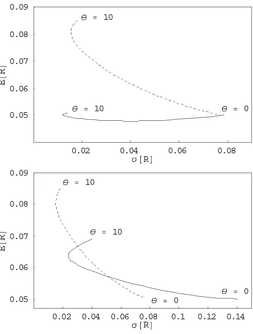
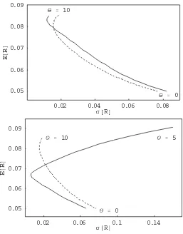
Figure 4: Basic immunization strategy returns
in the mean-standard deviation space
with different interest rate environments.
0.02 0.04 0.06 0.08
σ@RD 0.05
0.06 0.07 0.08 0.09
E
@
R
D
θ = 10
θ = 10
θ = 0
0.02 0.04 0.06 0.08 0.1 0.12 0.14
σ@RD 0.05
0.06 0.07 0.08 0.09
E
@
R
D θ = 10
θ = 10
θ = 0
θ = 0
Figure 4 plots the returns of the basic immunization strategy in the mean-standard deviation space for every horizon θ. Bond maturity is T = 10, and coupon rate is c = 0.1. For the top
figure, interest rate environment isΩ1(dashed line) andΩ2 (straight line). For the bottom figure,
Figure 5: Basic immunization strategy returns
in the mean-standard deviation space
with different bond characteristics.
0.02 0.04 0.06 0.08
σ@RD 0.05
0.06 0.07 0.08 0.09
E
@
R
D
θ = 10
θ = 0
0.02 0.06 0.1 0.14
σ@RD 0.05
0.06 0.07 0.08 0.09
E
@
R
D
θ = 5
θ = 10
θ = 0
Figure 5 plots the returns of the basic immunization strategy in the mean-standard deviation space for every horizon θ. Interest rate parameters areΩ1. For the top figure, bond maturity is T = 10, and coupon rate isc = 0.05. For the bottom figure, bond maturity isT = 5, and coupon
Figure 6: Duration-based strategies in the mean-standard deviation space:
The case for basic immunization strategy returns.
0.02 0.03 0.04
σ@RD 0.07
0.08
E
@
R
D
θ∗
MAC FW
STO
Figure 6 plots the returns of the basic immunization strategy in the mean-standard deviation space for every horizonθ. The respective positions of strategies based on traditional and stochastic
durations are highlighted. Interest rate environment isΩ1. Bond maturity isT = 10, coupon rate
Figure 7: Convergence of the Monte Carlo experiment.
2000 4000 6000 8000 10000n
0.0666 0.0668 0.067 0.0672 0.0674
mean
2000 4000 6000 8000 10000n
0.0018 0.0019 0.002 0.0021 0.0022 0.0023
stddev
2000 4000 6000 8000 10000n
3.6 3.8 4 4.2 4.4
Sharpe
Figure 7 plots the mean and standard deviation of returns as well as the Sharpe ratio as a function of the number of simulated sample paths. The dynamic immunization strategy is the one using the minimum variance duration. Interest rate environment isΩ1.Bond maturity isT = 5,
Fi
gure 8: Duration-based strategies in the mean-standard deviation space:
The case for dynamic immunization strategy returns.
0.002 0.004
σ@RD 0.065
0.075 0.085
E
@
R
D
Y10
θ∗ MAC
STO
Figure8 plots the returns of the dynamic immunization strategy in the mean-standard
[image:32.612.151.460.154.348.2]Tables
Table 1: Mean-variance analysis of the basic immunization strategy:
Different interest rate environments.
Min. var. Traditional durations Stochastic duration Macaulay Fisher-Weil duration
θ∗ θmac θfw θsto
Panel A: Interest rate parameters areΩ1
θ(years) 8.802 6.820 6.795 4.895
E (Rθ) (%) 8.062 7.326 7.316 6.642
σ (Rθ) (%) 1.538 2.055 2.066 3.059
Sharpe ratio 1.306 0.668 0.660 0.270 Panel B: Interest rate parameters are Ω2
θ(years) 9.102 7.043 7.070 5.167
E (Rθ) (%) 5.019 4.888 4.890 4.812
σ (Rθ) (%) 1.210 1.834 1.821 2.889
Sharpe ratio 0.765 0.367 0.371 0.156 Panel C: Interest rate parameters are Ω3
θ(years) 8.251 6.939 6.949 6.321
E (Rθ) (%) 6.366 6.011 6.014 5.859
σ (Rθ) (%) 2.375 3.314 3.302 4.131
Sharpe ratio 0.549 0.271 0.272 0.175
Table 2: Mean-variance analysis of the basic immunization strategy:
Different maturities and 10% coupon.
Min. var. Traditional durations Stochastic duration Macaulay Fisher-Weil duration
θ∗ θmac θfw θsto
Bond maturity isT = 3
θ(years) 2.872 2.620 2.620 2.510
E (Rθ) (%) 6.071 5.972 5.972 5.929
σ (Rθ) (%) 0.275 0.548 0.550 0.734
Sharpe ratio 1.747 0.760 0.757 0.531 Bond maturity isT = 5
θ(years) 4.673 4.038 4.034 3.611
E (Rθ) (%) 6.674 6.433 6.431 6.273
σ (Rθ) (%) 0.614 1.085 1.090 1.595
Sharpe ratio 1.432 0.646 0.642 0.369 Bond maturity is T = 10
θ(years) 8.802 6.820 6.795 4.895
E (Rθ) (%) 8.062 7.326 7.316 6.642
σ (Rθ) (%) 1.538 2.055 2.066 3.059
Sharpe ratio 1.306 0.668 0.660 0.270
For various bond maturities, Table 2 reports the duration (in years), the expected return (in percentage), the volatility (in percentage) and the Sharpe ratio of the associated basic immuniza-tion strategy. The Sharpe ratio is defined as in Table 1. Interest rate environment isΩ1. Coupon
Table 3: Mean-variance analysis of the basic immunization strategy:
Different maturities and 5% coupon.
Min. var. Traditional durations Stochastic duration Macaulay Fisher-Weil duration
θ∗ θmac θfw θsto
Bond maturity isT = 3
θ(years) 2.937 2.784 2.783 2.712
E (Rθ) (%) 6.091 6.030 6.030 6.001
σ (Rθ) (%) 0.163 0.361 0.362 0.497
Sharpe ratio 3.016 1.250 1.246 0.870 Bond maturity isT = 5
θ(years) 4.847 4.411 4.408 4.083
E (Rθ) (%) 6.725 6.556 6.555 6.431
σ (Rθ) (%) 0.397 0.834 0.838 1.313
Sharpe ratio 2.305 0.942 0.937 0.529 Bond maturity is T = 10
θ(years) 9.557 7.760 7.740 5.771
E (Rθ) (%) 8.315 7.624 7.617 6.909
σ (Rθ) (%) 1.172 2.080 2.094 3.331
Sharpe ratio 1.903 0.778 0.770 0.308
For various bond maturities, Table 2 reports the duration (in years), the expected return
Table 4: Mean-variance analysis of the dynamic immunization strategy:
Different maturities and 5% coupon.
Min. var. Traditional durations Stochastic duration Macaulay Fisher-Weil duration
θ∗ θmac θfw θsto
Bond maturity isT = 3
E (Rθ) (%) 5.958 5.958 5.958 5.958
σ (Rθ) (%) 0.111 0.113 0.113 0.114
Sharpe ratio 3.135 3.079 3.078 3.059 Bond maturity isT = 5
E (Rθ) (%) 6.679 6.680 6.680 6.681
σ (Rθ) (%) 0.208 0.215 0.215 0.218
Sharpe ratio 4.108 3.991 3.991 3.928 Bond maturity is T = 10
E (Rθ) (%) 8.423 8.429 8.429 8.435
σ (Rθ) (%) 0.407 0.431 0.431 0.458
Sharpe ratio 5.711 5.402 5.403 5.097
For various bond maturities (in years), Table 4 reports the expected return (in percentage), the volatility (in percentage) and the Sharpe ratio of the associated dynamic immunization strategy. The Sharpe ratio is defined as(E (Rθ) − y (θ)) /σ (Rθ) where y (θ) = −(1/θ) ln P (0, θ)is the
Table 5: Mean-variance analysis of the dynamic immunization strategy
under the Longstaff-Schwartz model:
Different maturities and 5% coupon.
Traditional durations Stochastic Macaulay Fisher-Weil duration
θmac θfw θsto
Bond maturity isT = 3
E (Rθ) (%) 6.270 6.270 6.270
σ (Rθ) (%) 0.095 0.095 0.097
Sharpe ratio 4.155 4.155 4.034 Bond maturity isT = 5
E (Rθ) (%) 6.948 6.948 6.948
σ (Rθ) (%) 0.187 0.187 0.194
Sharpe ratio 4.860 4.860 4.686 Bond maturity is T = 10
E (Rθ) (%) 8.666 8.666 8.666
σ (Rθ) (%) 0.428 0.428 0.460
Sharpe ratio 5.616 5.615 5.220
For various bond maturities (in years), Table 5 reports the expected return (in percentage), the volatility (in percentage) and the Sharpe ratio of the associated dynamic immunization strategy. The Sharpe ratio is defined as(E (Rθ) − y (θ)) /σ (Rθ) where y (θ) = −(1/θ) ln P (0, θ)is the