The comparative method in evolution-ary biology can be used to denote any and all uses of interspecific comparisons to draw evolutionary inferences (e.g., Ridley, 1983; Cheverud et al., 1985; Felsenstein, 1985; Grafen, 1989, 1992; Gittleman and Kot, 1990; Brooks and McLennan, 1991; Harvey and Pagel, 1991; Lynch, 1991; Martins and Garland, 1991; Carpenter, 1992b; Gittle-man and Luh, 1992; Pagel, 1992; Pagel and Harvey, 1992; Losos and Miles, 1994). Be-cause species usually will not represent in-dependent data points in the statistical sense, conventional parametric and
non-Syst.BIOI.42(3):265-292, 1993
PHYLOGENETIC ANALYSIS OF COVARIANCE BY
COMPUTER SIMULATION
THEODORE GARLAND, JR.,! ALLAN W. DICKERMAN,!,3 CHRISTINE M. JANIS,2 AND JASON A. JONES!
IDepartment of Zoology, University of Wisconsin, Madison, Wisconsin 53706, USA 2Program in Ecology and Evolutionary Biology, Division of Biology and Medicine, Brown University,
Providence, Rhode Island02912,USA
Abstract.-Biologistsoften compare average phenotypes of groups of species defined cladis-tically or on behavioral, ecological, or physiological criteria (e.g., carnivores vs. herbivores, social vs. nonsocial species, endotherms vs. ectotherms). Hypothesis testing typically is accomplished via analysis of variance (ANOVA) or covariance (ANCOVA; often with body size as a covariate). Because of the hierarchical nature of phylogenetic descent, however, species may not represent statistically independent data points, degrees of freedom may be inflated, and significance levels derived from conventional tests cannot be trusted. As one solution to this degrees of freedom problem, we propose using empirically scaled computer simulation models of continuous traits evolving along "known" phylogenetic trees to obtain null distributions ofFstatistics for AN-CaVA of comparative data sets. These empirical null distributions allow one to set critical values for hypothesis testing that account for nonindependence due to specified phylogenetic topology, branch lengths, and model of character change. Computer programs that perform simulations under a variety of evolutionary models (gradual and speciational Brownian motion, Ornstein-Uhlenbeck, punctuated equilibrium; starting values, trends, and limits to phenotypic evolution can also be specified) and that will analyze simulated data by ANCOVA are available from the authors on request. We apply the proposed procedures to the analysis of differences in home-range area between two clades of mammals, Carnivora and ungulates, that differ in diet. We also apply the phylogenetic autocorrelation approach and show how phylogenetically indepen-dent contrasts can be used to test for clade differences. All three phylogenetic analyses lead to the same surprising conclusion: for our sample of49species, members of the Carnivora do not have significantly larger home ranges than do ungulates. The power of such tests can be increased by sampling species so as to reduce the correlation between phylogeny and the independent variable (e.g., diet), thus increasing the number of independent evolutionary transitions available for study. [Allometry; behavioral ecology; body size; branch lengths; comparative method; com-puter simulation; home range; physiological ecology; statistics.]
parametric methods are inappropriate for hypothesis testing with interspecific data. Several explicitly phylogenetic statistical methods have therefore been developed. In addition to solving purely statistical problems, the incorporation of phyloge-netic information (topology, branch lengths) into analyses of patterns seen among living (and/ or extinct) species (e.g., phenotypic variation and covariation) sometimes allows inferences to be made concerning evolutionary processes (e.g., [co]adaptation, constraints, trade-offs, rates of evolution) (e.g., Huey and Bennett, 1987; Coddington, 1988; Lauder and Liem, 1989;
3Present address: Department of Ecology and Evo- Losos, 1990; Baum and Larson, 1991;
Gar-lutionary Biology, University of Arizona, Tucson, Ar- land et al., 1991; Garland, 1992; Miles and
izona85721,USA. Dunham, 1992).
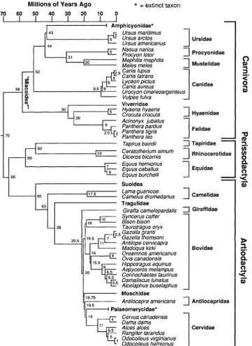
Most of the phylogenetically based "comparative methods" have focused on testing for character correlations, often with continuous traits such as body size, limb proportions, metabolic rate, or home-range area (Felsenstein, 1985, 1988; Grafen, 1989, 1992; Lynch, 1991; Martins and Gar-land, 1991; Garland et al., 1992; Gittleman and Luh, 1992; Pagel, 1992; and reviewed in Harvey and Pagel, 1991: chap. 5). In ad-dition to testing for character correlations, however, biologists often wish to compare mean phenotypes among groups of organ-isms defined on the basis of phylogenetic affinity or on behavioral, ecological, or physiological criteria. In comparative physiology, for example, analyses of vari-ance (ANOVAs) and analyses of covarivari-ance (ANCOVAs) (e.g., Tanner, 1949; Sokal and Rohlf, 1981; Packard and Boardman, 1988) are used routinely to compare metabolic rates among taxa (e.g., field metabolic rates of birds and mammals [Nagy, 1987]). Com-parative biochemists have compared in vitro enzyme activities of fishes that differ in feeding strategies and locomotor habits (e.g., Hochachka and Somero, 1984). At the chromosomal level, Burton et al. (1989) compared the nuclear DNA content of four families of bats. Many other examples can be found in behavioral ecology, including Barclay and Brigham's (1991) comparison by ANCOVA of frequency of echolocation calls of bats that differ in foraging mode and comparisons of phenotypes of animals with different diets, social systems, geo-graphic distributions, or habits (e.g., Mil-ton and May, 1976; Garland, 1983; Garland et al., 1988; Harvey and Pagel, 1991; Janis, in press). Sometimes such comparisons will fall strictly along phylogenetic lines. For the species listed in Figure 1, for example, the carnivores (Canidae, Hyaenidae, Feli-dae) and omnivores (Ursidae, Procyonidae, Mustelidae, Viverridae) fall within a lin-eage (order Carnivora) that separated about 70 million years ago from herbivores in the orders Perissodactyla and Artiodactyla (to-gether with Proboscidea, Hyracoidea, Sire-nia, and [cladistically speaking] Cetacea, the "ungulates"). Other comparisons might cut across clades.
Unless all of the species being compared
radiated more-or-Iess instantaneously from a common ancestor (a star phylogeny, e.g., Felsenstein, 1985: fig. 2; Martins and Gar-land, 1991: fig. 3a), their phenotypes prob-ably are not statistically independent. Har-vey and Pagel (1991:38-48) reviewed three biological reasons for lack of indepen-dence, which they termed time lags, phy-logenetic niche conservatism, and pheno-type-dependent responses to selection (see also discussions in Ridley, 1983; Cheverud et al., 1985; Felsenstein, 1985, 1988; Cod-dington, 1988; Grafen, 1989; Gittleman and Kot, 1990; Lynch, 1991). The time-lag rea-son is perhaps most intuitive. Once spe-ciation has occurred, it simply takes time for divergence to occur either as a result of random genetic drift or in response to natural selection for new phenotypes (Le., adaptation) (cf. McKinney, 1990b:l06). The statistical consequences of nonindepen-dent data points can include inflation of Type I error rates (due to overestimated degrees of freedom) when testing hypoth-eses, lowered power to detect significant relationships, and inefficient estimates of evolutionary parameters (e.g., Felsenstein, 1985, 1988; Grafen, 1989; Lynch, 1991; Mar-tins and Garland, 1991).
Conventional ANOVAs and ANCOVAs useFstatistics for hypothesis testing. Crit-ical values for F statistics are determined by reference to standard tabular values (e.g., Rohlf and Sokal, 1981: table 16), with de-grees of freedom determined by the num-ber of groups being compared and the total number of observations (e.g., species) in the data set. Unfortunately, the hierarchi-cal phylogenetic relationships of species within most comparative data sets make it difficult to know how many degrees of freedom actually obtain.
We therefore propose the use of empir-ically scaled computer simulations of char-acters evolving along "known"
phyloge-netic trees to obtain empirical F
1993 COMPARATIVE METHODS FOR ANOVA 267
Millions of Years Ago *
=
extinct taxon70 60 50 40 30 20 10 0
I I I I I I I I
Amphicyonidae*
43
2 Ursus maritimus
] Ursidae
5 Ursus arctos
44 Ursus americanus
Nasua narica ] Procyonidae
Procyon lotor
0
Mephitis mephitis
] Mustelidae
Melesmeles mセ
52 2 5Canis lupus
J
:::sセ 63' Canis latransgcaon pictus "
<-
0iii" anis aureus Canidae セ
58 n
9 Urocyon cinereoargenteus m
0
c:
Vulpes fulva(1)
qIセ Viverridae
30 Hyaena hyaena
] Hyaenidae
Crocuta crocuta Acinonyx jubatus
] Felidae
Panthera pardus
70 2 Panthera leoPanthera tigris
-c
(1)
Tapirus bairdii
:J
Tapiridae セ50
Ceratotherium simum ] Rhinocerotidae
iii-13
Diceros bicornis fn0
Equus hemionus
] Equidae
C.
7
Equus caballus m
6 n
66 Equus burchelli '<P+
Suoidea
m
17.5 Lamaセオ。ョゥ」ッ・ ] Camelidae
50 Came us dromedarius
43 Tragulidae
Giraffa camelopardalis
::J
GiraffidaeSyncerus caffer Bison bison
38 Taurotragus oryx
2 5Gazella granti
20.5 7 . Gazella thomsoni
»
Anti/ope cervicapra セ
Madoqua kirki Bovidae P+
Oreamnos americanus
Cr
Ovis canadensis C.
Hippotragus equinus m
Aepyceros melampus nP+
Connochaetes taurinus セ
Damaliscus lunatus m
Alcelaphus buselaphus
Moschidae
19.75
] Antilocapridae
19.5 Antilocapra americana
Palaeomerycidae*
Cervus canadensis Damadama
Alces alces Cervidae
Rangifer tarandus
1 Odocoi/eus virginianus
Odocoi/eus hemionus
FIGURE1. Hypothesis of phylogenetic relationships for 19 species of Carnivora and 30 species of ungulates
[image:3.464.53.415.34.532.2]42
methods would sample or reshuffle across the tips of a phylogeny, ignoring cladistic structure (cf. Maddison and Slatkin, 1991; Carpenter, 1992a); thus, it would not fully account for the phylogenetic hierarchy (Harvey and Pagel [1991:152-155] dis-cussed randomization tests that can be ap-propriately applied to phylogenetically in-dependent contrasts). Perhaps some sort of hierarchical resampling scheme could be devised, but computer simulation methods would seem to allow greater flexibility for exploring alternative models of evolution-ary change. In principle, the computer sim-ulation (or Monte Carlo) approach can be applied to hypothesis testing with any type of statistical test; Martins and Garland (1991) originally developed it for testing correlated evolution.
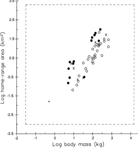
We illustrate the simulation approach with an analysis of differences in home-range area between two clades of mam-mals, the Carnivora (primarily carnivores but including some omnivores) and un-gulates (exclusively herbivores in the pres-ent subset of species) (Fig. 1). Differences in home range between trophic categories (e.g., Fig. 2) are of long-standing interest to behavioral and physiological ecologists. For mammals, herbivores tend to have smaller home ranges than do carnivores (Milton and May, 1976; Harestad and Bun-nell, 1979; Garland, 1983; Calder, 1984; Harvey and Pagel, 1991:30-31, 122; Dun-stone and Gorman, 1993; and refs. therein). In simple (and adaptive) terms, this differ-ence has been explained by the higher tro-phic level occupied by carnivores, which means that their foodHィ・イ「ゥカッイ・セI is more widely dispersed and offers fewer joules per unit home-range area than does the food of herbivores (plants). The data for the 49 species that we analyzed are part of a larger study (Garland, 1992; Garland et al., 1992; Garland and Janis, 1993; Janis, in press) and are used here primarily for heu-ristic purposes. The generality of our re-sults should be tempered by the knowl-edge that only a sparse sample of the diversity of living carnivores and herbi-vores is included. However, these 49 spe-cies do appear to represent an unbiased
sample, with respect to home-range area, of Carnivora and ungulates. Moreover, the same conclusion-that home-range area does not differ significantly between Car-nivora and ungulates-is reached when the data are analyzed by the proposed simu-lation methods, by phylogenetic autocor-relation procedures, and by an indepen-dent-contrasts approach. Our sample data also help point out the limitations of com-parative analyses in which phylogeny is perfectly confounded with the indepen-dent variable (diet, in the present case).
METHODS Specification of Phylogeny
All of the tests proposed herein require specification of the phylogenetic topology and branch lengths for the species under study. This requirement is consistent with those for phylogenetically based methods for estimating and testing evolutionary correlations (Felsenstein, 1985, 1988; Gra-fen, 1989, 1992; Harvey and Pagel, 1991; Lynch, 1991; Martins and Garland, 1991; Garland et al., 1992). To avoid circularity (but see de Queiroz, 1989: appendix 4), the phylogenetic information should be based on data other than and independent of the phenotypic characters to be studied (Fel-senstein, 1985, 1988; Brooks and Mc-Lennan, 1991; Harvey and Pagel, 1991; Martins and Garland, 1991; Sillen-Tullberg and Moller, 1993). The composite phylog-eny used here is depicted in Figure 1; its evidential support is presented in the Ap-pendix.
1993 COMPARATIVE METHODS FOR ANOVA 269
refs. therein). Because it is a random pro-cess with no constraints, Brownian motion change can sometimes yield periods of rap-id (almost punctuational) change as well as apparent trends over time (Lande, 1986; Bookstein, 1988: fig. 2).
In the context of phylogenetic simula-tions, Brownian motion can be imple-mented by drawing one random change for each branch segment from a normal distribution and rescaling the variance of the normal distribution in proportion to each branch segment. If branch lengths in units of time (or some other metric that varies among segments) are used, then a Brownian motion simulation is conven-tionally termed ugradual," to indicate that characters usually experience greater changes along longer branches. If, how-ever, all branch segments are set at 1, then the simulation can be termed uspeciation-al" (Rohlf et al., 1990). The concept behind a speciational model is that all change oc-curs in association with speciation events; setting all branch segments equal to 1 is simply a convenient way to simulate this process under Brownian motion. Martins and Garland (1991) termed such simula-tions upunctuational," but speciational is a preferable term because punctuational usually implies change occurring in only one daughter. Huey and Bennett's (1987) original implementation of a minimum-evolution (=squared-change parsimony of Maddison, 1991) algorithm for studying correlated evolution assumed speciational change. Martins and Garland (1991) and Maddison (1991; his weighted squared-change parsimony) generalized the Huey / Bennett algorithm for nonequal branch lengths (i.e., gradual Brownian motion evolution) (see also Garland et al., 1991).
Brownian motion evolution can be sim-ulated with our PC-based PDSIMUL com-puter program, which is similar to but more flexible than the CMSIMUL program of Martins and Garland (1991). The means, variances, and correlation of the bivariate distribution from which random changes are drawn (input distribution of Martins and Garland [1991]) can be user specified. By default, PDSIMUL and CMSIMUL set
variances of the input distribution such that simulated data sets (i.e., the phenotypes of the species at the tips of the phylogeny) will, on average, have variances equal to those of the real data set (see Martins and Garland, 1991). Because ANOVAs are based on relative amounts of variation within versus among groups, this scaling of vari-ance is immaterial for the analysis of data sets simulated under Brownian motion. (The same is true for analyses of correla-tions [Martins and Garland, 1991], al-though estimation of regression slopes does depend on the actual proportionality of variances of different characters.)
As many workers have emphasized, both the inference of phylogenetic trees them-selves and inferences about how other characters have evolved along given trees depend crucially on the model of change assumed (e.g., Felsenstein, 1985, 1988; Fri-day, 1987; Rohlf et al., 1990; Harvey and Pagel, 1991; Maddison, 1991; Maddison and Slatkin, 1991; Martins and Garland, 1991). Although Brownian motion models of character change lead to relatively simple analyses, many other models are possible, at least some of which are probably more biologically realistic (Felsenstein, 1985, 1988; Martins and Garland, 1991). The evo-lutionary relevance of P values derived from simulated data depends on the real-ism of the simulation conditions (cf. Stan-ley et al., 1981; Carpenter, 1992a, 1992b). Accordingly, we have also developed sev-eral other simulation models (available in PDSIMUL), all of which allow some pa-rameters to be empirically scaled.
One model is the Ornstein-Uhlenbeck (OU) process, which has been described by Felsenstein (1988:464):
Uhlenbeck& Ornstein defined a diffusion process that has a linear [force] returning [a particle] to a central point. At any instant the expected change is toward that point, at a rate proportional to the particle's distance from the point. The change var-ies around this in a way otherwise typical of Brownian motion.
ge-netic drift, with natural selection acting as an elastic band. The
au
process "could also serve as the model for the wanderings of an adaptive peak in the phenotypic space, where the optimum remains within a rel-atively confined region" (Felsenstein, 1988: 464-465). An important feature of anau
model of character change "is that it grad-ually I'forgets' past history" (Felsenstein, 1988:465). The stronger the force tending to return species' phenotypes to their start-ing point, the more rapidly a set of species will become statistically independent-the more rapidly history will be "forgotten."PDSIMUL implements the
au
process as follows. Beginning at the bottom of the specified tree, a bivariate change is drawn for each branch segment. This random movement of the trait, similar to Brownian motion, occurs in conjunction with a ten-dency for the trait to be "pulled" towards a user-specified adaptive peak. At any time, the strength of this pulling is proportional to (1) the distance between the trait and the peak and (2) the decay constant, also user specified. A decay constant of zero would be equivalent to simple Brownian motion. An infinitely large decay constant would mean that a lineage's phenotype would decay back to the adaptive peak along each branch segment.If the adaptive peak is specified to be the same as the starting values of the traits (at the root of the phylogeny), then stabilizing selection is being modeled by the
au
de-cay constants. If the position of the adap-tive peak is specified to be different from the starting values of the traits, then the phenotypic peak will move to this new po-sition, either monotonically or stochasti-cally, as specified in PDSIMUL; here, both directional and stabilizing selection are be-ing modeled. Under gradualau
evolu-tion, both the random movement of the trait and its movement due to the pull of the adaptive peak are modeled to take place continuously in time (or whatever the units of branch length) along each branch seg-ment. In speciationalau
evolution, the random movement is modeled to take place instantaneously at speciation events and then to decay back towards the specifiedadaptive peak along branch segments of unit length. (Mathematical details are in the PDSIMUL documentation.)
Another evolutionary model is punctu-ated equilibrium, in which character change is allowed only at speciation events and only in one of the two daughter lin-eages. This model agrees with the original descriptions of punctuated equilibrium, in which genetic and phenotypic change is postulated to occur only in small periph-eral populations that bud off from a large "parent" species (Eldredge and Gould, 1972; Gould and Eldredge, 1977). Simula-tion algorithms by Raup and Gould (1974) and by Colwell and Winkler (1984) have followed this model.
N one of the models described above pro-vide for any explicit limits on how large or small a character can evolve to be. In many cases, however, one may be willing to specify limits to the realistic range of character values (see also discussions in Friday, 1987). For example, the smallest mammal has probably never been less than 1-2 g. The largest known terrestrial mam-mal is the fossilBaluchitherium(also known
asIndricotheriumorParaceratherium),which
probably weighed no more than about 15,000 kg (mean adult mass about 11,000 kg, M. Fortelius and J. Kappelman, pers. comm.; but see Economos, 1981; Alexan-der, 1989). Various explanations for such patterns are possible, such as "reflection inside the borders of a fitness range" that is "suggestive of ... boundaries of a more or less fixed ecological niche" (Bookstein, 1988:381, 389) (see also McKinney, 1990a, 1990b). More generally, limits to pheno-typic evolution may be attributable to any type of biomechanical, developmental, physiological, or genetic "constraint" (e.g., Rose et al., 1987; Werdelin, 1987; Garland, 1988; Pease and Bull, 1988; Lauder and Liem, 1989; Vrba, 1989; Charlesworth, 1990; McKinney, 1990b; Weber, 1990; Zelditch et al., 1990; Janson, 1992; Losos and Miles, 1994; also, Schmidt-Nielsen [1984] and Al-exander [1989] discuss possible physical limits on Baluchitherium).
documen-1993 COMPARATIVE METHODS FOR ANOVA 271
tation), and we have chosen one of the simplest for purposes of illustration (termed "Replace" in PDSIMUL). If a change to be drawn would exceed the spec-ified limits, it was replaced with a new change.
Use of the foregoing limits procedure, as with our implementation of the OU model, will lead to variances for the tip data that may be smaller than those for the real data. It is not the differences in vari-ances per se that affect ensuing F distri-butions, but rather the nature and inter-actions of the algorithms implementing the OU process and/or the limits to how far traits can evolve. Even with limits im-posed, however, the variances of simulated data can generally be made to match those of real data by increasing the parameter for expected variances at the tips in the PDSIMUL program.
We have used limits of 0.03 and 15,000 kg for body mass (see Fig. 2). The former is the lower end of the size range of the least weasel, Mustela rixosa, the smallest living member of the Carnivora; the latter is the approximate upper size of
Baluchithe-rium, the largest fossil ungulate (M.
For-telius and
J.
Kappelman, pers. comm.). We used limits of 0.001 and 2,000 km2for(non-migratory) home-range area, based on in-spection of values presented in Harestad and Bunnell (1979) and Goszczynski (1986) (e.g., the largest reported home range for a member of the Carnivora is for the wol-verine, Gulo gulo, about 1,000-1,500 km2
).
All simulations were done on a loglo scale; thus, specified limits were -1.5229 and 4.1761 for body mass and -3.0 and 3.3010 for home range. We used starting values of -0.3010 (loglo of 0.5 kg) for body mass and -1.8036 (on the loglo scale) for home-range area. This body mass is the approx-imate size of the last common ancestor of Carnivora and ungulates, assuming
Protun-gulatum to be representative (see
Appen-dix). The home-range value was estimated by a least-squares linear regression through the origin fitted to standardized indepen-dent contrasts (Felsenstein, 1985; Garland et al., 1992), yielding a slope of 1.2616 (r = 0.7212). This line was positioned through
the point (2.0051, 1.1057), which repre-sents the independent contrasts estimates for the root node, and extrapolated to -0.3010 (=loglo of 0.5 kg). Forcing through the values estimated for the root node is appropriate because these values are also estimates of the overall group means, weighted by phylogeny; in the present case, they are quite similar to means calculated in the conventional way (1.9037 and 1.1666, respectively). Maddison (1991) showed an-alytically that the independent contrasts estimates for the basal node are also iden-tical to the squared-change parsimony or minimum evolution (Huey and Bennett, 1987; Martins and Garland, 1991) estimates (both are computed by the CMSINGLE program of Martins and Garland [1991]). These starting values are outside the range exhibited in the real data set for living spe-cies-such a pattern is not uncommon for mammals (e.g., MacFadden, 1986: fig. 4 on horses).
Creating Empirical Null Distributions for Hypothesis Testing
Once the phylogenetic topology, branch lengths, and model of evolutionary change have been specified, then a large number of computer simulations are run, typically 1,000. For each set of simulated tip data, various statistics (e.g., mean, variance, sums of squares, correlation) can be computed for each group specified a priori. These em-pirically scaled null distributions form the basis for hypothesis testing.
We have written computer programs to read in sets of simulated tip data, calculate various statistics, and output the results to standard ASCII files. These ASCII files can then be analyzed with conventional sta-tistical packages.
F ratio for the real data set (which can be obtained from PDSINGLE or from a con-ventional statistical package) exceeded the upper 95th percentile of the empirical null distribution, we would conclude that the two clades differed significantly in mean body mass. Conventional statistics were done with SPSSjPC+ version 3.1.
Available Programs
All of the programs discussed herein (named "PD_" as an acronym for "Phe-notypic Diversity") are available from the authors on request.
PDTREE graphically displays trees and allows editing, including transforms of both branch lengths (see Garland et al., 1992) and phenotypic data. It will translate file format between that compatible with the Martins and Garland (1991) programs (_.INP) and that used with PDSINGLE and PDANOVA (_.PDI).
PDSIMUL simulates gradual and specia-tional Brownian motion, Ornstein-Uhlen-beck, or punctuated equilibrium evolution of two continuous characters (with speci-fied correlation) along a specispeci-fied phylog-eny. It also allows specification of limits to how far phenotypes can evolve. It can be used with trees that contain multifurcating nodes (except with punctuated equilibri-um).
PDSINGLE analyzes a single set of real data for two continuous characters and computes descriptive statistics (means, me-dians, variances, correlation), ANOVA, ANCOVA with one variable as covariate, and Levene's test for relative variation (Schultz, 1985).
PDANOVA analyzes multiple sets of simulated data, as produced by PDSIMUL or CMSIMUL. It performs the same com-putations as in PDSINGLE and writes a series of ASCII files as output, which can then be entered into conventional statis-tical packages for computation of empirical null distributions of F statistics, etc.
RESULTS
To illustrate the proposed method, we consider data on home-range area in re-lation to body mass for 49 species of
mam-mals. The current working phylogeny for these species is shown in Figure 1 and de-scribed in the Appendix; phenotypic data are listed in Table 1.
Hypothesis Testing with Computer-Simulated Null Distributions Figure 2 shows a scattergram of home-range area versus body mass (data pre-sented in Table 1), suggesting that carni-vores and omnicarni-vores as a group (n = 19; all in the order Carnivora) have larger home ranges than do herbivores (n = 30 ungulates in the orders Artiodactyla and Perissodactyla). A conventional ANCOVA (Table 2) of the log-transformed data yields an F statistic for the diet (=clade) effect of 23.97, which is highly significant with the nominal 1 and 46 degrees of freedom and a critical value of 4.049 for a = 0.05. The pooled within-groups slope from the AN-CaVA is 0.997, which is also highly sig-nificant(F = 47.40, df = 1,46,P < 0.001). Because omnivores do not appear distinct with respect to home range, we have lumped them with carnivores for simplic-ity.
1993 COMPARATIVE METHODS FOR ANOVA 273
TABLE 1. Body mass and home-range areas for 19 species of Carnivora and 30 ungulates. These are the same 49 species analyzed by Garland and Janis (1993) for correlations between maximal running speed and limb proportions.
Body mass Home range
Species (kg) (km2) Reference
Ursus maritimus 265.0 115.6 DeMaster and Stirling, 1981; Schweinsburg and Lee, 1982
Ursus arctos 251.3 82.8 Janis, in press
Ursus americanus 93.4 56.8 Janis, in press
N asua narica 4.4 1.05 Kaufmann, 1962; Kaufmann et al., 1976
Procyon lotor 7.0 1.14 Harestad and Bunnell, 1979
Mephitis mephitis 2.5 2.5 Harestad and Bunnell, 1979; Bjorge et al., 1981
Meles meles 11.6 0.87 Janis, in press
Canis lupus 35.3 202.8 Harestad and Bunnell, 1979
Canis latrans 13.3 45.0 Janis, in press
Lycaon pictus 20.0 160.0 Janis, in press
Canis aureus 8.8 9.1 Janis, in press
Urocyon cinereoargenteus 3.7 1.1 Janis, in press
Vulpes fulva 4.8 3.87 Harestad and Bunnell, 1979
Hyaena hyaena 26.8 152.8 Janis, in press
Crocuta crocuta 52.0 25.0 Janis, in press
Acinonyx jubatus 58.8 62.1 Janis, in press
Panthera pardus 52.4 23.2 Janis, in press
Panthera tigris 161.0 69.6 Janis, in press
Panthera leo 155.8 236.0 Janis, in press
Tapirus bairdii 250.0 2.0 Eisenberg et al., 1990 (estimate from density)
Ceratotherium simum 2,000.0 6.65 Janis, in press
Diceros bicornis 1,200.0 15.6 Janis, in press
Equus hemionus 200.0 35.0 Janis, in press
Equus caballus 350.0 22.5 Janis, in press
Equus burchelli 235.0 165.0 Janis, in press
Lama guanicoe 95.0 0.5 Franklin, 1982; Cajal, 1991
(estimate from territory size and densities)
Camelus dromedarius 550.0 100.0 Kohler-Rollefson, 1991
Giraffa camelopardalis 1,075.0 84.6 Janis, in press
Syncerus caffer 620.0 138.0 Janis, in press
Bison bison 865.0 133.0 Janis, in press
Taurotragus oryx 511.0 87.5 Janis, in press
Gazella granti 62.5 20.0 Janis, in press
Gazella thomsonii 20.5 5.3 Janis, in press
Antilope cervicapra 37.5 6.5 Janis, in press
Madoqua kirki 5.0 0.043 Janis, in press
Oreamnos americanus 113.5 22.75 Janis, in press
Ovis canadensis nelsoni 85.0 14.33 Harestad and Bunnell, 1979
Hippotragus equinus 226.5 80.0 Janis, in press
Aepyceros melampus 53.25 3.8 Janis, in press
Connochaetes taurinus 216.0 75.0 Janis, in press
Damaliscus lunatus 130.0 2.2 Janis, in press
Alcelaphus buselaphus 136.0 5.0 Janis, in press
A ntilocapra americana 50.0 10.0 Harestad and Bunnell, 1979; Janis, in press
Cervus canadensis 300.0 12.93 Harestad and Bunnell, 1979
Dama dama 55.0 1.3 Putnam, 1988
Alces alces 384.0 16.1 Harestad and Bunnell, 1979
Rangifer tarandus 100.0 30.0 Janis, in press
Odocoileus virginianus 57.0 1.96 Harestad and Bunnell, 1979
42
3.5
2.5
セ
N
E
1.5 ..Y"--"
o
(])
(5 0.5
(])
CJ"l
C
o
7 -0.5
(])
E
o...c CJ"l -1.5 o
-I
-2.5
r---l
! l
I I
! l
I I
!
Nセᄋo
lI • 0 I
! .X.O: 0 l
I • I
! セ Cb 0 I
1 & 0 I
! • 0 l
I 0 0 0 l
! • 0 0 l
I X 0 I
! 0 0 0 l
I セ X 0 I
! l
I 0 I
! l
I I
! l
I I
! 0 l
I I
! * I
I I
! l
I l
! l
I I
L セ セ セ
4
-1 -3.5 MKMM⦅セ⦅K⦅⦅MMMMMlM⦅⦅KMMMlNNNM⦅K⦅MセM⦅K⦅MNlNNM⦅⦅⦅KMMMMlNM⦅K⦅MMMj
-2
a
1 2 3 [image:10.459.88.365.41.339.2]Log body mass (kg)
FIGURE 2. Log-log relationship between home-range area and body mass in 30 species of ungulates (0) and 19 species of Carnivora(e= carnivores; X= omnivores[Ursus arctos, Ursus americanus, Nasua narica, Procyon lotor, Mephitis mephitis, Meles meles]) (data from Table 1). The solid line is a least-squares linear regression fitted to standardized independent contrasts and positioned through the bivariate mean (.) estimated by independent contrasts. For simulations, the asterisk(*)represents the ancestral starting value (-0.3010 for loglo body mass, -1.8036 for loglo home-range area) and the dashed line represents the specified limits to evolution (30 g and 15,000 kg for body mass, 0.001 and 2,000 km2for home range).
adjusted for body size, does not differ sig-nificantly between clades. Our conclusion about a possible group difference is thus different when phylogenetic noninde-pendence is incorporated through com-puter simulation techniques. However, the correlation between home-range area and body mass is highly significant under ei-ther model of change (Table 2; critical val-ues were 17.02 and 15.20 for gradual and speciational change, respectively, with F
=
47.40 for the real data).
Gradual and speciational Brownian mo-tion models are among the simplest that can be employed for simulating correlated evolution of continuous characters, but they are not necessarily the most realistic.
measure-TABLE 2. Analysis of covariance comparing loglo home-range areas of members of the Carnivora (including both carnivores and omnivores) with those of ungulates (all herbivores), with loglo body mass as the covariate. Critical values for F statistics and associated significance levels are presented for conventional tabular values (from harmonic interpolation, Rohlf and Sokal, 1981: table 16), which would be strictly appropriate onlyifall species radiated instantaneously from a common ancestor (a star phylogeny), and based on analyses of data simulated along the phylogeny shown in Figure 1 under different models of character change. For all five simulations, the starting phenotypic values (at the root of the phylogeny) were 0.5 kg for body mass and 0.031623 km2for home-range area, and limits on character evolution were set as 0.03-15,000 kg for body mass and 0.01-1,000 km2for home-range area. Values for covariate and explained are not relevant for the group difference hypothesis being tested. Last three simulations were done with a correlation of 0.7212, as indicated by an independent contrasts analysis of the real data (so the F for real data is exceedingly unlikely to be judged "different" at P < 0.05).
Brownian motion
Gradual with
Conventional Ornstein- Punctuated
tabular Gradual3 Speciationalb limits and trendC Uhlenbeckd equilibriume
Source of Sum of Mean Critical Critical Critical Critical Critical Critical
variation squares df square F value P value P value P value P value P value P
Main effect 8.48 1 8.48 23.97 4.049 <0.001 68.07 0.229 52.61 0.186 76.19 0.215 47.22 0.147 56.62 0.192
Covariate 16.77 1 16.77 47.40 4.049 <0.001 17.02 0.004 15.20 0.001 177.28 0.552 151.71 0.545 561.69 0.998
Explained 17.40 2 8.70 24.58 3.199 <0.001 43.60 0.153 31.93 0.104 158.07 0.742 113.79 0.707 359.31 0.999
Error 16.28 46 0.35
Total 33.67 48 0.70
3Mean means (±2 SE) were 1.900 ± 0.024 and 1.162 ± 0.030 for loglO body mass and loglO home-range area, respectively; mean variances were 0.502 ± 0.018 and 0.709 ±
0.024; mean Pearson correlation was -0.008 ± 0.020. Pseudorandom number seed was 2.
bMean means were 1.908 ± 0.030 and 1.149 ± 0.038, respectively; mean variances were 0.501 ± 0.016 and 0.701 ± 0.022; mean correlation was 0.016 ± 0.018. Seed was 3. Speciational evolution (Rohlf et al., 1990) was referred to as punctuational by Martins and Garland (1991); this model allows equal probability of change in both daughter species rather than only in one daughter, as was originally specified for punctuated equilibrium.Itis mathematically equivalent to gradual change along a phylogeny with all branch lengths set to be equal.
CMean means were 1.886 ± 0.026 and 1.145 ± 0.030, respectively; mean variances were 0.489 ± 0.016 and 0.681 ± 0.022; mean correlation was 0.695 ± 0.012. Seed was 6.
dMean means were 1.881 ± 0.020 and 1.134 ± 0.024, respectively; mean variances were 0.395 ± 0.010 and 0.575 ± 0.016; mean correlation was 0.703 ± 0.010. Seed was 4.
[image:11.632.24.611.193.292.2]42
3.5
2.5
セ
N
E
1.5 ..Y"--"
o
(])
o
0.5(])
CJ"l
C
o セ -0.5
(])
E
o
...c CJ"l -1.5 o
....J
-2.5
r---l
! l
I I
! l
I I
! l
I • I
! , 0 X l
I • I
! • •
80
lI セ I
! ッセ 0 l
I 0 0 I
! 0 セ 0 l
I 0 Q) I
! セL 0 セ l
I • X 0 I
! 0 l
I I
! • 0 _ l
I • セ I
! 0 I
I 0 I
! l
I I
! * l
I I
! l
I I
! l
I I
L _ _ _ _ _ _ _ _ _ _ _ _ _ _ _ _ _ _ _ _ _ _ _ _ Nセ __.J
4
a
1 2 3Log body mass (kg)
-1 -3.5TMMNNNiMMMNjMMMlNNNMMMMiMMMMャNMMKMセM⦅ヲ⦅MNNNiMM⦅K⦅MMGMMMK⦅⦅MMMMG
[image:12.457.88.366.39.336.2]-2
FIGURE 3. Example of computer-simulated home range and body mass data (from "Gradual with limits and trend" column in Table 2). The distribution from which changes were drawn was scaled so as to yield, on average, simulated tip data with variances similar to those of the real data (as listed in Table 1). The correlation of the distribution was set to be 0.7212, as indicated by analysis of standardized independent contrasts. Starting point for simulations is indicated by the asterisk(*)(see text and Fig. 2 caption). Limits to how far the characters could evolve (dashed lines; see text and Fig. 2 caption) were set using the "Replace" option of the PDSIMUL program. Other symbols are as in Figure 2. For this data set, theFstatistics from the ANCOVA are 139.05 for body mass and 22.88 for diet (carnivores plus omnivores vs. herbivores).
ments of lower second lower molar lengths and using equations in Janis [1990]). For the 1,000 simulated speciational data sets, the maximum and minimum loglo body mass values were 5.697 (497,737 kg) and -2.523 (0.003 kg). Clearly, realistic limits can be exceeded even though variances of the simulated data are, on average, the same as those of the real data (the default in both PDSIMUL and CMSIMUL); similarity of variances does not guarantee similarity of minima or maxima. Moreover, starting simulations at the mean loglo body mass of the values exhibited by the extant species in the data (1.9037
=
80.1 kg) is very un-realistic for mammals living 70 millionyears ago. We therefore also simulated data under more complicated and, presumably, more realistic models.
mono-1993 COMPARATIVE METHODS FOR ANOVA 277
tonically to shift (see documentation ac-companying PDSIMUL, which also allows stochastic trends) the mean of the character distributions from the specified starting values (see Fig. 2) to the mean of the real tip data. The third of these conditions sim-ulates a gradual trend for increasing body mass (cf. McKinney, 1990b) and home-range size. Such a model has been termed "diffusion with drift" by Berg (1983), where drift refers to the force pulling the particles (species) in a particular direction (see Mc-Kinney, 1990b:84-87). Figure 3 shows one example of data simulated under this mod-el. Under this model, the critical value for the group effect was 76.19, yielding P =
0.215.
The fourth model in Table 2 uses the Ornstein-Uhlenbeck process (see Felsen-stein, 1988). The following parameters were used in PDSIMUL: (1) the correlation was set at 0.7212; (2) the same limits to phe-notypic evolution were set; (3) the position of the adaptive peak, initially at the start-ing values, was increased monotonically ("Final Means" in PDSIMUL) to yield tip data with means similar to those of the real data; and (4) "Decay Constants" (the strength of the "spring" mimicking sta-bilizing selection in the OU process) were set to 1.0 x 10⁻⁸ for both traits. Here, the critical value for a = 0.05 is lower, F =
47.22, but still too high to indicate a sig-nificant difference in Carnivora and un-gulate home ranges (P = 0.147).
The final model in Table 2 is punctuated equilibrium, in which change occurs only at speciation events and only in one daughter, chosen randomly by PDSIMUL. The same starting values and limits to evo-lution were used, and the correlation of evolutionary changes was again set to 0.7212. Final Means were set to 4.45 and 4.65 for loglo body mass and loglo home-range area, respectively, which were the values determined by trial and error to yield realistic tip means (see Table 2 foot-notes). This model yielded a critical value of F=56.62 and an insignificant P= 0.192. Regardless of the simulation model em-ployed, we cannot reject the null hypoth-esis of no significant difference in
home-range area between Carnivora and ungu-lates for our sample of 49 species. The apparent difference in Figure 2-and com-monly accorded ecological and evolution-ary significance-is not very unusual when judged against a null model that includes both chance (as in conventional statistics) and phylogeny.
Phylogenetic Autocorrelation
Gittleman and Kot's (1990; Gittleman and Luh, 1992) phylogenetic autocorrelation programs were applied by H.-K. Luh to the data of Table 1. The transformation expo-nent for branch lengths,a, was estimated as 3.550 for loglo body mass and 4.006 for loglo home-range area; autocorrelation co-efficients were estimated as 0.65 and 0.32, and the proportions of variance explained by phylogeny (true R2) were 0.607 and 0.148, respectively. These parameter esti-mates were used in producing putatively phylogeny-free residuals. Figure 4 pre-sents a scatterplot of these residuals: the ANCOVA yielded F statistics of 47.41 for body mass (df = 1,44, P
<
0.001) and 0.58 for the clade effect (df=
1,44, P=
0.46) (two degrees of freedom are lost for esti-mating the a's used to transform branch lengths). Again, omnivores do not form a distinct group (cf. Fig. 2).278
0 0
セ
0
•
0 0x o x o· x
.0
00
0 x
•
0o
.
セ
x CD
•
6.
0 0o
. 0 0
o 0
.t>
o
•
o
1.5
o (1)
o
-0.5(1)
CJl C
o
7 -1.5
(1)
E
o
...c
CJl-2.5
o
-.J
-3.5-i---L----+---L.----f---'---+---I---i
-2.5 -1.5 -0.5 0.5 1.5
[image:14.457.78.388.36.259.2]Log body mass (kg)
FIGURE 4. Putatively phylogeny-free residuals of loglO home-range area and loglO body mass (phylogeny from Fig. I, data from Table 1) from a phylogenetic autocorrelation analysis (Gittleman and Kot, 1990). The ANCOVA of these residuals indicates no significant difference in mass-corrected home-range areas between herbivores(0)and carnivores(e)plus omnivores (X) (P= 0.46).
231) described an appropriate two-tailed test (modified for the present context):
value of single observation
- i of test distribution t =
-s 5D of test distribution·[(n
+
1)/n]0.5'where the test distribution is the distri-bution of all standardized contrasts except the basal contrast and n is the number of contrasts in the test distribution (n = 47 here). Because the direction of subtraction of contrasts is arbitrary, the mean of the test distribution is zero and the sign of the basal contrast is irrelevant. Also, the vari-ance of contrasts is computed as the simple sum of the squared contrasts, divided by n - 1 (see Garland et al., 1992: appendix 3). Applying this test to contrasts for our data on loglo body mass (from Table 1), we obtain
t
=
0.000170098=
1.372s 0.000122639. [(47
+
1) /47]0.5 ' with degrees of freedom n - 1 = 46. The critical value for atdistribution with df=46is 2.0125 fora = 0.05.We therefore
con-elude that the basal contrast is not unusual and hence that the two clades do not differ in mean body mass (P > 0.16).
1993 CaMPARATIVE METHODS FOR ANOVA 279
セ 0.0006
c
o
L o
o
•
o
x__
--•
•
o
--•
--•
o
o o
_ - --0
00
•
.. -=-_ - -
l)--(])
E
0.0004o
..c c
en
0.0002o
L C
o
o "0
(])
N
"0 L
.g
-0.0002c
o
Vi
0.00006 0.00012 0.00018 0.00024
Standardized contrast in body mass
-0.0004 +---.1....---i_ _- - . J ._ _-+_ _---L..._ _- i -_ _....L-_ _+-_----J
o
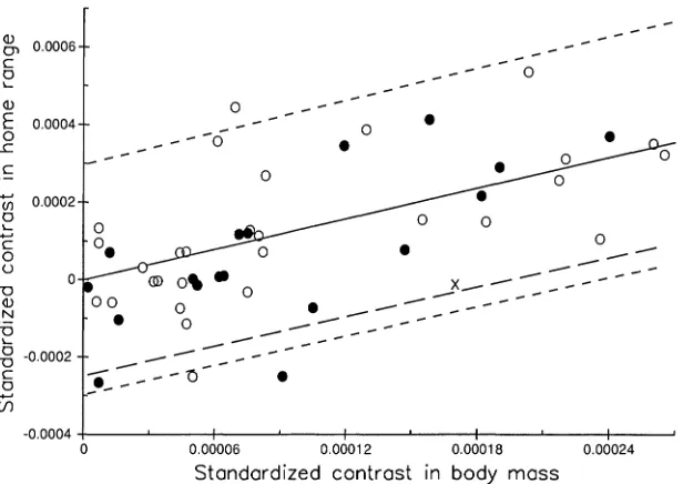
FIGURE5. Bivariate scatterplot of 48 standardized independent contrasts inャッセャo home-range area and loglo
body mass (redrawn from Garland et al., 1992: fig. 5a). Contrasts within Carnivora(e)and the ungulates(0)
are shown, along with the basal contrast (X). In this figure, body mass contrasts have been ""positivized" (Garland et al., 1992), and the signs of home-range contrasts changed accordingly. Solid line is least-squares linear regression through the origin for the 47 nonbasal contrasts (slope= 1.3171,r2
= 0.544,F= 54.90, P < 0.0001). Short dashed lines are the two-tailed 95% prediction interval; long-dashed line is the one-tailed 95% prediction interval (although not immediately obvious from this graph, these prediction intervals become wider farther away from the origin) (formulas from Neter et al., 1989:167-170). The basal contrast falls within these intervals, which indicates no significant difference in home-range area between Carnivora and ungulates.
= 47). As illustrated in Garland et al. (1992: fig. 4) for a 43-species data set, branch lengths for home-range area provide more even standardization if they are log trans-formed. A reanalysis of Figure 5 with log-transformed branch lengths for home-range area (not shown) yields a qualita-tively identical conclusion.
DISCUSSION
Analysis of variance and covariance, in-cluding multiple regression with dummy variables (Sokal and Rohlf, 1981; Neter et al., 1989), are often applied in comparative analyses of cross-species data (e.g., Schoe-ner, 1968; Turner et al., 1969; Milton and May, 1976; Harestad and Bunnell, 1979; Harvey and Clutton-Brock, 1981; Garland, 1983; Christian and Waldschmidt, 1984; Goszczynski, 1986; Nagy, 1987; Garland et al., 1988; Burton et al., 1989; Bunnell and Harestad, 1990; Barclay and Brigham, 1991;
Harvey and Pagel, 1991; Janis, in press). Such methods are powerful and general and are available in most statistics pack-ages. However, the F statistics obtained from the ANOV
AI
ANCOVA of compara-tive data cannot properly be judged for sig-nificance against conventional tabular val-ues (e.g., Rohlf and Sokal, 1981: table 16) because species' phenotypes generally are not statistically independent, which leads to overestimation of degrees of freedom. We have therefore proposed the use of em-pirically scaled, computer-simulated data to obtain "phylogenetically correct" or "PC" distributions ofFstatistics for testing hypotheses of differences between clades or other groups.Conclusions about Home-Range Area and Diet
[image:15.457.84.392.36.254.2]42
areas of19 members of the Carnivora (car-nivores plus om(car-nivores) with those of 30 ungulates, all of which are herbivores. Three different phylogenetically based tests agree: when judged by statistical tests that include both chance and phylogeny as part of the null hypothesis, ungulates do not have significantly smaller home ranges than do members of the Carnivora. What might explain this surprising result?
First, home-range area may actually be unrelated to diet, which is conceivable if, for example, carnivores have higher di-gestive efficiencies or perhaps higher for-aging efficiencies than do herbivores (cf. Harestad and Bunnell,1979; Garland, 1983; Calder, 1984; Goszczynski, 1986; Bunnell and Harestad, 1990; Harvey and Pagel, 1991:30-31, 122; Dunstone and Gorman, 1993). However, (nonphylogenetic) stud-ies of other groups of mammals and of oth-er voth-ertebrates have genoth-erally indicated sig-nificant covariation between diet and home range (Schoener, 1968; Turner et al., 1969; Milton a11d May, 1976; Harestad and Bun-nell,1979; Harvey and Clutton-Brock, 1981; Christian and Waldschmidt, 1984; Gomp-per and Gittleman,1991; and refs. therein). We suspect that a broader data base might indicate that herbivorous mammals have significantly smaller home ranges.
Second, our test may have inadequate power to detect a significant difference. In the present data set, diet is perfectly con-founded with phylogeny (see Fig. 1and Table 1); the two dietary groups fallon either side of the root. In a maximum-par-simony reconstruction of diet evolution in this group of mammals, irrespective of the true ancestral state, only one dietary tran-sition has occurred-at the base of the tree. Intuitively, this confounding may yield low statistical power.
Statistical power can be increased in sev-eral ways, including increasing sample size. It may be more efficient to add data from other clades of mammals, rather than just increase sample sizes within Carnivora and ungulates, thus increasing the number of independent dietary transitions available for a study. Power could also be increased by obtaining diet information on a contin-uous scale, such as percent meat in diet.
This would allow (multiple) correlation or regression tests for an association between diet and home-range size (e.g., using in-dependent contrasts). Reduction in biolog-ical "noise" in the data through the use of additional covariates other than body mass, such as latitude, group size, or habitat type (cf. Milton and May, 1976; Gompper and Gittleman,1991; Janis, in press), could also increase power. Finally, more powerful statistical methods might be possible. In future studies, we plan to use computer simulation (cf. Martins and Garland, 1991) to compare the power of the three ap-proaches applied here plus that of Lynch (1991), modified for ANOVA.
Assumptions, Limitations, and Potential of the Simulation Approach
1993 COMPARATIVE METHODS FOR ANOVA 281
and Luh, 1992). Our PDSIMUL program can simulate data along unresolved trees by initially entering an arbitrarily resolved tree structure into PDTREE and then set-ting some internode branch lengths equal to zero.
Although unresolved nodes are easily incorporated into simulations, the relative lengths of the branches above and below a polytomy will affect the critical values obtained. If branches between a polyto-mous node and its descendants are set to be relatively short, then critical values will be conservative because the descendants are being treated as close relatives, ex-pected to be relatively similar phenotypi-cally (as if degrees of freedom were re-duced). Conversely, if branches between a polytomous node and its descendants are set to be relatively long, descendants will be treated as relatively statistically inde-pendent, yielding liberal critical values. These effects should be kept in mind when using arbitrary branch lengths. Other ways to deal with polytomies include simply omitting species whose relationships are uncertain or performing the analysis with several alternative topologies (see also Gra-fen, 1992; Pagel, 1992; Sillen-Tullberg and Moller, 1993; Losos and Miles, 1994).
In the limit, we may have a completely unresolved tree-a star phylogeny sensu Martins and Garland (1991)-with all spe-cies derived from a single explosive radi-ation (cf. Felsenstein, 1985: fig. 2). Some groups of living species may actually de-rive from such a quick radiation, as has been suggested for African cichlid fishes (Mayden, 1986). If the group under study is accurately represented as a star phylog-eny-a "hard" polytomy in Maddison's (1989) terminology-then conventional tabular F statistics can be used for the
AN-OVAs/ ANCOVAs. It might also be possi-ble to choose for study only taxa whose phylogenetic relationships are almost star-like (e.g., one species from each of the deep branches of a phylogeny or several pop-ulations of a single species [cf. Garland et al., 1992:26-27]).
A hypothetical star phylogeny can also be used to test whether our simulation methods yield the correct Type I error rates.
We used PDTREE to "unresolve" the phy-logeny of Figure 1 into a star and then used PDSIMUL to simulate gradual Brownian motion evolution of two characters with zero correlation 1,000 times. These data were then analyzed with PDANOVA, and the numbers of F statistics exceeding the nominal critical values for a
=
0.05 (from harmonic interpolation of Rohlf and Sokal, 1980: table 16) were counted. The Type I error rates were 0.048, 0.039, and 0.045 for the main effect, covariate, and explained, respectively (cf. Table 2). In a second trial, using a different random number seed (10 instead of 1), Type I error rates were 0.057, 0.044, and 0.046, respectively. Thus, our simulation and analysis procedures yield-ed acceptable Type I error rates.In our example, estimates of branch lengths in units of absolute time were available (relative time would be compu-tationally equivalent for our purposes). But temporal branch lengths are only appro-priate if the characters being studied evolve as by pure gradual Brownian motion, with evolutionary rates stochastically equal over time and across lineages. What is really needed is branch lengths in units of ex-pected variance of change (Felsenstein, 1985; Martins and Garland, 1991). Branch lengths can be obtained in a variety of ways (Grafen, 1989; Harvey and Pagel, 1991; Martins and Garland, 1991; Pagel, 1992; Walton, 1993; Martins, in press), and Gar-land et al. (1992; also GarGar-land, 1992) dis-cussed tests to check the statistical adequa-cy of branch lengths as well as ways to transform them to improve their statistical properties (see also Grafen, 1989). If trans-formation of branch lengths is indicated, then simulations could be done with the transformed branch lengths. Our current programs allow only bivariate simulations along a single set of branches. N onethe-less, the ability to set variances, limits, peak shifts, etc., separately for each trait (in PDSIMUL) allows, in effect, different branch lengths to be imposed during sim-ulations.
be handled by using batch files to read simulated data sets into commercial statis-tics packages, such as SAS, SPSS, or SY-STAT. Multiple range comparisons with ordered predictions should also be possi-ble (cf. Gaines and Rice, 1990). Compari-sons of variances of groups of species are possible using Levene's test (e.g., Schultz, 1985), which is an ANOVA performed on absolute deviations of individual species' values from their within-group means or medians (Garland and Dickerman, in prep.). The simulation approach can be ap-plied to any statistical test so long as one analyzes both the real and simulated data in an identical fashion.
Alternative Models of Character Evolution
The utility of P values derived from com-puter simulation depends on the realism of the simulation model (e.g., Stanley et al., 1981). We therefore used several dif-ferent models, some with parameters set empirically, based on the data being ana-lyzed and / or the fossil record. If scaling parameters are derived from the data being analyzed, as in our use of an independent contrasts regression to estimate a starting value for home range (see Methods and Fig. 2), then the resulting P values may be slightly liberal.
A gradual Brownian motion model of character change is reasonable under the neutral theory of phenotypic evolution and for some types of selection (Felsenstein, 1985, 1988; Charlesworth, 1990; Lynch, 1990; and refs. therein), but many other options are possible (see Felsenstein, 1988; Rohlf et al., 1990; Martins and Garland, 1991; and refs. in Slowinski and Guyer, 1989a, 1989b). PDSIMUL also allows spe-ciational change, the Ornstein-Uhlenbeck process, punctuated equilibrium, trends, and limits to phenotypic evolution. Mod-els that incorporate species selection or
Isorting (Vrba, 1989; Gould, 1990) would be
of interest; they would require coincident simulation of both the tree and the char-acters evolving along it (cf. Rohlf et al., 1990; Vida et al., 1990; Vogi and Wagner, 1990; Maddison and Slatkin, 1991). Until
we know more about micro- and macro-evolutionary processes (Endler and Mc-Lellan, 1988; Felsenstein, 1988; Vrba, 1989; Gould, 1990), it is prudent to simulate char-acter evolution under several models (cf. Rohlf et al., 1990; Martins and Garland, 1991)-a type of sensitivity analysis-and check for consistency in final results (cf. Losos, 1990; Garland et al., 1991; Sillen-Tullberg and Moller, 1993; Walton, 1993; Martins, in press).
Our implementation of punctuated equilibrium has some interesting proper-ties. Because the tree topology is fixed and no extinction is allowed, the starting val-ues at the root node will always be present at the tips in the simulated data. In fact, the phenotypes at every node will be rep-resented at the tips. Thus, in our example, although we could obtain simulated data with realistic means (see Table 2), both dis-tributions of means were left skewed be-cause at least one tip species was always "anchored" at the root value, leading to variances that were too high, even with upper limits to evolution also imposed. Moreover, the Pearson correlation of tip data was higher than desired (Table 2 foot-notes). Perhaps it would be more appro-priate to model punctuated equilibrium by simulating the phylogeny simultaneously. Application of both speciational (cf. Martins and Garland, 1991; Garland et al., 1992) and punctuated equilibrium models assumes that all branching points within the clade under study have been sampled, or at least that they have been sampled randomly or proportionately along all branches; otherwise, simulation along the phylogeny for only the species being com-pared (e.g., the present 49 species) may be misleading. Notwithstanding this and oth-er indications of apparently unrealistic as-sumptions in some of our simulations, the conclusion regarding statistical signifi-cance is robust (Table 2).
Alternative Approaches for Phylogenetic ANCOVA
1993 COMPARATIVE METHODS FOR ANOVA 283
fashion. First, Lynch (1991) derived from quantitative genetics (treating phylogeny as analogous to a pedigree) a maximum likelihood-based method for estimating evolutionary correlations and phylogenet-ic "heritabilities." In principle, this meth-od could be extended to estimate mean
dif-ferences among clades or among
ecologically defined groups. Computer programs to do so are not yet available (M.
Lynch, pers. comm.). .
Second, Gittleman and Kot's (1990) ap-plication of Cheverud et al.'s (1985; see also Gittleman, 1991; Miles and Dunham, 1992) phylogenetic autocorrelation method can produce residuals that are putatively free from phylogenetic effects. Harvey and Pa-gel (1991:137) questioned the logic of phy-logenetic autocorrelation methods, be-cause they discard a portion of the total variation observed among species: "poten-tially the majority of the variation is as-signed to phylogenetic components and is . .. not ... used to test questions about function and adaptation." Philosophical reservations aside, our use of putatively phylogeny-free residuals in a convention-al ANCOVA (Fig. 4) yielded quconvention-alitatively the same result as did the computer sim-ulation and independent contrasts meth-ods.
Third, Felsenstein's (1985) method of standardized independent contrasts can be applied to comparisons of group means (see also Grafen, 1989, 1992; Martins, in press). Standardized independent contrasts are phenotypic differences between sister spe-cies or nodes divided by the square root of the patristic distance between them: they indicate "rates" of change in subclades of a tree (Garland, 1992). Thus, our applica-tion to the comparison of phenotypic means of two sister clades actually tests for a sig-nificantly higher "rate" of evolution at the point when the two clades diverged than at any time during evolutionary change within either. However, because the basal contrasts are entirely inferred from values for living species, the ultimate inference must be about the weighted mean values of the two samples of species; that is, an extreme basal standardized contrast is
in-terpretable as a difference in weighted mean phenotype for the two clades (see Fig. 5).
For comparison of two clades for a single trait (contra Fig. 5), such as body mass, a basic nonparametric approach is possible. After ranking the absolute values of all standardized independent contrasts, one can compute the simple probability of the basal contrast being as extreme as ob-served. For example, the probability of the basal contrast being the most extreme of 48 contrasts (derived from 49 species) would be 1/48
=
0.020833; the probability of its being one of the three most extreme contrasts would be 1/48+
1/48+
1/48=
0.0625. For the data in Table 1, the basal body mass contrast is the 11 th greatest; the probability of a ranking this extreme is 0.22917. We could also rank the residual home-range contrasts, computed from a re-gression fitted to all 48 contrasts (as op-posed to a line fitted to just 47 contrasts as shown in Fig. 5). If we do so, the basal contrast is the fourth smallest (P=0.08333). Another strategy would be to regress the absolute values of independent contrasts (not standardized) on their standard de-viations (square roots of sums of branch lengths), omitting the one contrast of in-terest, and compute a one-tailed 95% con-fidence interval for a new value for the regression (probably constrained through the origin; see Garland, 1992). If the basal contrast fell outside the confidence inter-val, this could be interpreted as indicating a significant difference in clade means.
284
of 0/1 dummy variables could be used (e.g., Sokal and Rohlf, 1981; Neter et aI., 1989). From a strict (multiple) regression per-spective, only the residuals need to be checked carefully for normality, homosce-dasticity, etc. (Grafen, 1989, 1992; Garland et aI., 1992). The statistical properties of contrasts for categorical or ordered vari-ables may, however, differ between those involving two tips (e.g., where all differ-ences are either zero or unity) and those involving interior nodes, where differ-ences get "smeared" across multiple con-trasts (M. D. Pagel, pers. comm.). If cate-gorical variables are employed with multivariate techniques such as principal components analysis, it is especially im-portant to verify that branch lengths yield adequate standardization (Garland et aI., 1992) and/or that the standardized con-trasts are multivariate normal. In principle, categorical variables might even be used as dependent variables in regressions, but residuals often will behave poorly and Type I error rates may be compromised (e.g., Wu, 1986). Methods such as logistic regression are more appropriate (A. Grafen, pers. comm.).
Often, categorical variables represent coarse information about what is actually an underlying continuous variable (e.g., Moller, 1991:885). A carnivore-herbivore dichotomization, for example, can be viewed as a crude substitute for percent meat in diet. For our example data set, we can rescore diet as a three-category ordered variable (herbivores
=
0, omnivores=
1, carnivores = 2), compute standardized contrasts, and perform a multiple regres-sion of home-range contrasts on both body mass and diet contrasts. This procedure yields only six non-zero diet contrasts, al-though all 48 are properly analyzed (cf. Garland et aI., 1992), and the partial F sta-tistic for diet contrasts (controlling for body mass) is insignificant (F=
0.696, df=
1,46, P=
0.4086) (residuals from the multiple regression appear to behave adequately).Independent contrasts can also be used to compare a single species to a group of other species. Ecological physiologists, for example, often study species living in
"ex-treme" environments in the hope of find-ing particularly clear examples of adapta-tion (Bartholomew, 1987; Garland and Adolph, 1991). Often, the "exemplar" spe-cies is compared with the "norm" shown by a set of other species. A classic and fre-quent example of this approach (e.g., McNab, 1992) is to compare the metabolic rate of a single species with a 95% confi-dence interval for a nonphylogenetic re-gression of metabolic rate on body mass. To be phylogenetically correct, such anal-yses could be done with independent con-trasts, similar to our comparison of the bas-al contrast to bas-all other within-clade contrasts (Fig. 5).
ACKNOWLEDGMENTS
We thank R. Chappell, J. Clobert, D. Bauwens, J. Felsenstein, J. L. Gittleman, A. Grafen, A. R. Ives, G. C. Mayer, M. D. Pagel, and various other colleagues for helpful discussions and J. M. Cheverud, A. Larson, J. B. Losos, and M. M. Miyamoto for comments on the manuscript. H.-K. Luh kindly analyzed the data with the phylogenetic autocorrelation programs of Gittleman and Luh (1992). This study was supported by N.S.F. grants BSR-9006083, BSR-9146864 (Research Experiences for Undergraduates), and BSR-9157628 (P.Y.I.) to T.G.
REFERENCES
ALEXANDER, R. M. 1989. Dynamics of dinosaurs and other extinct giants. Columbia Univ. Press, New York.
ALLARD, M. W., M. M. MIYAMOTO, L. JARECKI, F. KRAUS, AND M. R. TENNANT. 1992. DNA systematics and evolution of the artiodactyl family Bovidae. Proc. Natl. Acad. Sci. USA 89:3972-3976.
ARCHIBALD, J. D. In press. Archaic ungulates ("Con-dylarthra").InEvolution of Tertiary mammals of North America (C. M. Janis, K. M. Scott, and L. L. Jacobs, eds.). Cambridge Univ. Press, Cambridge, England.
BARCLAY, R. M. R., AND R. M. BRIGHAM. 1991. Prey detection, dietary niche breadth, and body size in bats: Why are aerial insectivorous bats so small? Am. Nat. 137:693-703.
BARTHOLOMEW, G. A. 1987. Interspecific comparison as a tool for ecological physiologists. Pages 11-37 in New directions in ecological physiology (M. E. Feder, A. F. Bennett, W. W. Burggren, and R. B. Huey, eds.). Cambridge Univ. Press, Cambridge, England.
BASKIN, J. A. 1982. Tertiary Procyonidae (Mammalia: Carnivora) of North America. J. Vertebr. Paleontol. 2:71-93.
1993 COMPARATIVE METHODS FOR ANOVA
285
Teritary mammals of North America (C. M. Janis, K. M. Scott, and L. L. Jacobs, eds.). Cambridge Univ. Press, Cambridge, England.
BAUM, D. A., AND A. LARSON. 1991. Adaptation re-viewed: A phylogenetic methodology for studying character macroevolution. Syst. Zool. 40: 1-18. BENNETI, D. K. 1980. Stripes do not a zebra make.
Syst. Zool. 29:272-287.
BERG, H. C. 1983. Random walks in biology. Prince-ton Univ. Press, PrincePrince-ton, New Jersey.
BJORGE, R. R., J. R. GUNSON, AND W. M. SAMUEL. 1981. Population characteristics and movements of striped skunks(Mephitis mephitis) in central Alberta. Can. Field-Nat. 95:149-155.
BOOKSTEIN, F. L. 1988. Random walk and the bio-metrics of morphological characters. Evol. BioI. 23: 369-398.
BROOKS, D. R., AND D. A. McLENNAN. 1991. Phylog-eny, ecology, and behavior. A research program in comparative biology. Univ. Chicago Press, Chicago. BUNNELL, F. L., AND A. S. HARESTAD. 1990. Activity budgets and body weight in mammals: How sloppy can mammals be? Pages 245-305inCurrent mam-malogy, Volume 2 (H. H. Genoways, ed.). Plenum, New York.
BURTON, D. W., J. W. BICKHAM, AND H. H. GENOWAYS. 1989. Flow-cytometric analyses of nuclear DNA content in four families of neotropical bats. Evo-lution 43:756-765.
CAJAL, J. 1991. An integrated approach to the man-agement of wild camelids in Argentina. Pages
305-321 inLatin American mammalogy: History, bio-diversity, and conservation (M. A. Mares and D. S. Schmidly, eds.). Univ. Oklahoma Press, Norman. CALDER, W. A. 1984. Size, function and life history.
Harvard Univ. Press, Cambridge, Massachusetts. CARPENTER, J. M. 1992a. Random cladistics.
Cladis-tics 8:147-153.
CARPENTER, J. M. 1992b. Comparing methods. Cla-distics 8:191-196.
CHARLESWORTH, B. 1990. Optimization models, quantitative genetics, and mutation. Evolution 44: 520-538.
CHEVERUD, J. M., M. M. Dow, AND W. LEUTENEGGER. 1985. The quantitative assessment of phylogenetic constraints in comparative analyses: Sexual di-morhpism in body weight among primates. Evo-lution 39:1335-1351.
CHRISTIAN, K. A., AND S. WALDSCHMIDT. 1984. The relationship between lizard home range and body size: A reanalysis of the data. Herpetologica 40:68-75.
CHURCHER, C. S.,AND M. L. RICHARDSON. 1978. Equi-dae. Pages 379-422inEvolution of African mam-mals (V. J. Maglio and H. B. S. Cooke, eds.). Harvard Univ. Press, Cambridge, Massachusetts.
CODDINGTON, J. A. 1988. Cladistic tests of adapta-tional hypotheses. Cladistics 4:3-22.
COLWELL, R. K.,AND D. W. WINKLER. 1984. A null model for null models in biogeography. Pages
344-359 in Ecological communities, conceptual issues and the evidence (D. R. Strong, Jr., D. Simberloff,
L. G. Abele, and A. B. Thistle, eds.). Princeton Univ. Press, Princeton, New Jersey.
CRONIN, M. 1991. Mitochondrial-DNA phylogeny of deer (Cervidae). J. Mammal. 72:533-566. CROWLEY, P. H. 1992. Resampling methods for
com-putation-intensive data analysis in ecology and evolution. Annu. Rev. Ecol. Syst. 23:405-447. OEMASTER, D. P., ANDI.STIRLING. 1981. Ursus
mar-itimus.Mamm. Species 145:1-7.
DE QUEIROZ, K. 1989. Morphological and biochem-ical evolution in the sand lizards. Ph.D. Disserta-tion, Univ. California, Berkeley.
DUNSTONE, N., AND M. GORMAN (eds.). 1993. Mam-mals as predators. Symp. Zool. Soc. Lond. 65 (in press).
ECONOMOS, A. C. 1981. The largest land mammal. J. Theor. BioI. 89:211-215.
EISENBERG, J. F., C. P. GROVES, AND K. MACKINNON. 1990. Tapirs. Pages 598-608inGrzimek's encyclo-pedia of mammals, Volume 4 (S. P. Parker, ed.). McGraw-Hill, New York.
ELDREDGE, N., AND S. J. GOULD. 1972. Punctuated equilibria: An alternative to phyletic gradualism. Pages 82-115inModels in paleobiology (T. J. M. Schopf, ed.). Freeman, Cooper and Co., San Fran-cisco.
ENDLER, J. A., AND T. McLELLAN. 1988. The process of evolution: Toward a newer synthesis. Annu. Rev. Ecol. Syst. 19:395-421.
FELSENSTEIN, J. 1985. Phylogenies and the compar-ative method. Am. Nat. 125:1-15.
FELSENSTEIN, J. 1988. Phylogenies and quantitative characters. Annu. Rev. Ecol. Syst. 19:445-471. FLYNN, J. J. In press. Early Cenozoic Carnivora
(UMiacoidea"). In Evolution of Tertiary mammals of North America (C. M. Janis, K. M. Scott, and L. L. Jacobs, eds.). Cambridge Univ. Press, Cambridge, England.
FLYNN, J. J., AND H. GALIANO. 1982. Phylogeny and Early Tertiary Carnvora, with a description of a new speices ofProtictisfrom the Middle Eocene of north-western Wyoming. Am. Mus. Novit. 2725:1-64. FLYNN, J. J., N. A. NEFF, AND R. H. TEDFORD. 1988.
Phylogeny of the Carnivora. Pages 73-116inThe phylogeny and classification of the tetrapods, Vol-ume 2 (M. J. Benton, ed.). Clarendon Press, Oxford, England.
FRANKLIN, W. L. 1982. Biology, ecology, and rela-tionship to man of the South American camelids. Pages 457-489 in Mammalian biology in South America, Volume 6 (M. A. Mares and H. H. Gen-oways, eds.). Special Publ. Ser., Pymatuning Lab-oratory of Ecology, Univ. Pittsburgh, Pittsburgh, Pennsy1vania.
FRIDAY, A. 1987. Models of evolutionary change and the estimation of evolutionary trees. Oxf. Surv. Evol. BioI. 4:61-88.
GAINES, S. D., AND W. R. RICE. 1990. Analysis of biological data when there are ordered expecta-tions. Am. Nat. 135:310-317.
286 42
GARLAND, T., JR. 1988. Genetic basis of activity me-tabolism.I.Inheritance of speed, stamina, and an-tipredator displays in the garter snakeThamnophis sirtalis.Evolution 42:335-350.
GARLAND, T., JR. 1992. Rate tests for phenotypic evo-lution using phylogenetically independent con-trasts. Am. Nat. 140:509-519.
GARLAND, T., JR., AND S. C. ADOLPH. 1991. Physio-logical differentiation of vertebrate populations. Annu. Rev. Eco1. Syst. 22