Abstract
This paper describes the concept of multiple input multiple output (MIMO) system using polarization diversity that can enhance the channel capacity and increase the data output performance of the system. The microstrip antenna array is designed, fabricated and measured at the desired operating frequency for this measurement. Computer Simulation Technology (CST) sotware is used to design and simulate the microstrip antenna array. The simulation and measurement data results are compared and discussed. The fabricated microstrip antenna is used to develop the Radio Frequency (RF) MIMO test bed system. The system measurement was conducted in Microwave Laboratory at Faculty of Electronic and Computer Engineering, University Technical Malaysia Melaka with the operating frequency of 2.4 GHz. The spatial diversity and polarization diversity are applied in measurement campaign to investigate the performance of the wireless MIMO channel. The data obtained from the measurement was post-processed using MATLAB sotware in order to calculate the MIMO channel capacity. The analysis focused on the efect of the MIMO channel capacity due to the proposed measurement setup conigurations. The channel capacity was increased from 0.03 b/s/Hz to 0.09 b/s/Hz when polarization diversity is applied at both transmiter and receiver.
Keywords: MIMO System, MIMO Channel Capacity, Polarization Diversity.
The InvesTIgaTIon of PolarIzaTIon DIversITy In
MIMo sysTeM aT 2.4 ghz
M.z.a. abd aziz
1, M.K.a. rahim
2, M.f.a Kadir
1, M.K. suaidi
1,
z. Daud
1, M.h. Jamaluddin
11
Faculty of Electronic and Computer Engineering,
Universiti Teknikal Malaysia Melaka,
Hang Tuah Jaya, 76100 Durian Tunggal, Melaka Malaysia
2
Faculty of Electrical Engineering, Universiti Teknologi Malaysia,
81310 Skudai, Johor, Malaysia
Email: [email protected], [email protected]
I. InTroDUCTIon
Wireless communication systems become more important as they provide lexibility and application user friendly. The technology of mobile communication and wireless local network (WLAN) are expending at fast rate which is to assure that the end users reach a maximum data transfer and a get a beter quality of service. The Multiple Input Multiple Output (MIMO) system is introduced to improve the communication system without having an additional transmit power or larger bandwidth, this because the MIMO system can utilize the multipath propagation.
The use of antenna arrays in wireless communication systems provides many advantages. For example channel capacity can be greatly increased with increasing antenna array at both link [1] [2].
t d ) d uter e and to e g
distributed through the channel [3].
Figure1 : Classic Wireless Communication Figure1 : Classic Wireless Communication
MIMO channel describes the connection between the transmiters and receiver. The MIMO channel models can be divided into the non-physical and physical models [4][5].
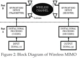
Generally the MIMO system can be divided into two parts, which the irst part is the digital signal processing (DSP) and representing as Part a in Figure 2. The second part is radio frequency (RF) device and representing as Part B in Figure 2. [6].
portant user friendly. ireless hich m data transfer ltiple the any e the t. stems channel capacity can h link
Figure 2: Block Diagram of Wireless MIMO System Figure 2: Block Diagram of Wireless MIMO
System
This paper will discuss and analyzed the channel capacity efect to the wireless MIMO channel by using polarization diversity. The various conigurations of polarization diversity applied at the both sides of transmiter and receiver has been studied.
II. DIversITy In MIMo
sysTeM
Recently the diversity technique was used to enhance the wireless system. The propagation mechanism was an issued that degraded the wireless performance. So, the diversity technique was used in order to improve the wireless transmission by transmiting the information multiple
times. Thus, increased the probability at receiver end where at least one of the signals will be received correctly [7].
The spatial diversity was referred as the technique that space apart the distance between the antennas[8]. The spatial diversity was been implemented in order to enhance the system performance. Such in [9], reported that the space diversity (spatial diversity) was an eicient technique for picocell (indoor to indoor) environment by achieving 14 b/s/Hz and 16 b/s/Hz capacities in 80% of the cases for 4x4 antenna coniguration which spatial diversity created decorrelated signals between the antennas. The spatial diversity can be realized such in [10] implemented the spatial diversity by setup the antenna spacing to λ/2, λ and 2λ. In research[10], to increased the number of antennas elements, polarization has recently been accepted as the cost efective solution and also to obtain more uncorrelated channels.
vertically polarized with neighboring ones orthogonal to each other.
III. MIMo sysTeM
MeasUreMenT
The measurement setup is done to characterize the channel in diferent environments and scenarios. The scenario can be Line of Sight (LOS), Non Line of Sight (NLOS) and obstructed Line of Sight (OLOS) [15]. As the transmiter and receiver have under no circumstance visibility, it is considered as NLOS scenario. For the LOS scenario is via versa of the NLOS scenario. As example of LOS scenario, the transmiter and receiver were located in the hallway which has visibility to each other’s [8]. Such in [12], the NLOS can be accomplished by placing the transmiter and receiver at two adjacent laboratories.
So, the environment can also be described as indoor, outdoor, and outdoor to indoor or in anechoic chamber. Basically, the measurement for indoor environment is done in building. Such in [15], the measurement is conducted in building that is typically modern oice building which is constructed with steel, concrete, dry walls, glass window and wooden door. As the [8] reported, the measurement is also conducted in building which the concrete is used to make loor and ceiling. The plasterboard with metal studs is used to make the walls.
Iv. MIMo Channel
CorellaTIon CoeffICIenT
Channel correlation between transmiter and receiver is calculated. Correlation coeicient is a measured of the linear relationship between transmiter and receiver [16]. Strong LOS usually considered as low-rank channel matrix and it will provide correlation between transmiter and receiver [17].
Thus, the mathematical equation that described the MIMO system can be expressed as Equation (1). x represents as the input signal and y represent as the output signal.
an be ersity by
λ λ λ rch
elements, polarization and
input signal and y represent
y = H x + n (
where H in Equation (1) sy
⎟⎟ ⎟ ⎟ ⎟
⎠ ⎞
⎜⎜ ⎜ ⎜ ⎜
⎝ ⎛
ρ
ρ
ρ
ρ
ρ
ρ
ρ
ρ
ρ
ρ
ρ
ρ
ρ
ρ
ρ
ρ
ρ
σ
σM x N
λ λ λ
al.
(1)
IMO channel
⎟⎟ ⎟ ⎟ ⎟
⎠ ⎞
⎜⎜ ⎜ ⎜ ⎜
⎝ ⎛
ρ
ρ
ρ
ρ
ρ
ρ
ρ
ρ
ρ
ρ
ρ
ρ
ρ
ρ
ρ
ρ
ρ
σ
σM x N
where H in Equation (1) symbolized for
the MIMO channel matrix and n was the noise in the system. The size of the MIMO channel matrix was depending on the number of transmits and receives antenna. Therefore, the Equation (2)
shows the MIMO channel matrix, H. N
represented as the number of transmiting antennas and M represent as the number of receiving antennas.
λ λ λ
use ta [12], a O LHCP. The larization er as the
he n be
receiving antennas.
H =
⎟⎟ ⎟ ⎟ ⎟
⎠ ⎞
⎜⎜ ⎜ ⎜ ⎜
⎝ ⎛
yx
ρ
ρ
ρ
ρ
ρ
ρ
ρ
ρ
ρ
ρ
ρ
ρ
ρ
ρ
ρ
ρ
43 42 41
34 33 32 31
24 23 22 21
11 13 12 11
ρ is the correlation coefficient between
σ
σM x N
λ λ λ
⎟⎟ ⎟ ⎟ ⎟
⎠ ⎞
⎜⎜ ⎜ ⎜ ⎜
⎝ ⎛
ρ
ρ
ρ
ρ
ρ
ρ
ρ
ρ
ρ
ρ
ρ
ρ
ρ
ρ
ρ
ρ
(2)
ρ tween the output
σ
σM x N
ρyx was the correlation coeicient
between the output signals and input signals. The correlation coeicient can be expressed as Equation (3). covyx was covariance between output power and input power. While σyy and σxx were variance of output power, y and input power, x irrespectively. The interval of the correlation coeicient was from +1 to -1.
(3)
phase. For complex correlation, it used amplitude or power with same to the power correlation [18].
x y
complex = ,
ρ
x y
envelope= ,
ρ
2 2 ,x y power =ρ
(
)
⎭ ⎬ ⎫ ⎩ ⎨ ⎧ ⎟⎟⎠ ⎞ ⎜⎜⎝ ⎛ ⎟ ⎠ ⎞ ⎜ ⎝ ⎛ + = ρ ρ∑
= ⎜⎜⎝⎛ + ⎟⎟⎠⎞ = λ λ =ρ
=ρ
=ρ
(6)(
)
⎭ ⎬ ⎫ ⎩ ⎨ ⎧ ⎟⎟⎠ ⎞ ⎜⎜⎝ ⎛ ⎟ ⎠ ⎞ ⎜ ⎝ ⎛ + = ρ ρ∑
= ⎜⎜⎝⎛ + ⎟⎟⎠⎞ = λ λ =ρ
(4)=
ρ
(5)=
ρ
(
)
⎭ ⎬ ⎫ ⎩ ⎨ ⎧ ⎟⎟⎠ ⎞ ⎜⎜⎝ ⎛ ⎟ ⎠ ⎞ ⎜ ⎝ ⎛ + = ρ ρ∑
= ⎜⎜⎝⎛ + ⎟⎟⎠⎞ = λ λv. Channel CaPaCITy
analysIs
MIMO channel capacity depends heavily on the statistical properties and antenna element correlations of the channel [19]. MIMO channel capacity is quantiies the maximum bit rate allowed by channel without error transmission [20]. Channel capacity is deine by
= ρ = ρ = ρ
(
)
⎭⎬⎫ ⎩ ⎨ ⎧ ⎟⎟⎠ ⎞ ⎜⎜⎝ ⎛ ⎟ ⎠ ⎞ ⎜ ⎝ ⎛ + = H NtMIMO E I Nt HH
C log2 det ρ (
where (.)H is the Hermitian operator which defi
ρ
∑
= ⎜⎜⎝⎛ + ⎟⎟⎠⎞ = λ λ =ρ
=ρ
=ρ
(
)
⎭ ⎬ ⎫ ⎩ ⎨ ⎧ ⎟⎟⎠ ⎞ ⎜⎜⎝ ⎛ ⎟ ⎠ ⎞ ⎜ ⎝ ⎛ += ρ (7)
ρ
∑
= ⎜⎜⎝⎛ + ⎟⎟⎠⎞ = λ λ Where (.)H is the hermitian operatordeined by transposed conjugate matrix,
E{.} is the expectation, ρ is signal
to noise ratio (SNR) and INt is is an n*m identity matrix. MIMO capacity increase by increasing angle spread factor for LOS and NLOS scenarios [21]. By calculating the eigenvalue of channel, capacity of the MIMO system is presented as:
=
ρ
=ρ
=ρ
(
)
⎭ ⎬ ⎫ ⎩ ⎨ ⎧ ⎟⎟⎠ ⎞ ⎜⎜⎝ ⎛ ⎟ ⎠ ⎞ ⎜ ⎝ ⎛ + = ρ ρ∑
= ⎜⎜⎝⎛ + ⎟⎟⎠⎞ =min{ , }1 0 2 . 1 . 1 log M N i s N N E C λ (
Where E /N presents the ratio of sig
λ =
ρ
=ρ
=ρ
(
)
⎭ ⎬ ⎫ ⎩ ⎨ ⎧ ⎟⎟⎠ ⎞ ⎜⎜⎝ ⎛ ⎟ ⎠ ⎞ ⎜ ⎝ ⎛ + = ρ ρ∑
= ⎜⎜⎝⎛ + ⎟⎟⎠⎞ = λ (8)al energy to no ing antenna and λ
Where ES/N0 presents the ratio of signal energy to noise energy, n and m is transmiting and receiving antenna and λ is the eigenvalue.
vI. MeasUreMenT seT UP
Figure 3 shows the typical MIMO system. Eight units of 2×2 rectangular microstrip
patch array antennas were ited at
transmiter and receiver. The do symbol
represents the inter element spacing also known as antenna spacing. Meanwhile, the measurement was conduct in indoor environment with Line of Sight (LOS) condition. The system operating frequency was 2.4 GHz with noise loor was -76 dBm.
on of rrelation = ρ ) = ρ ) =
ρ (6)
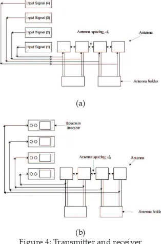
( ) ⎭⎬⎫ ⎩ ⎨ ⎧ ⎟⎟⎠ ⎞ ⎜⎜⎝ ⎛ ⎟ ⎠ ⎞ ⎜ ⎝ ⎛ + = ρ ρ ∑= ⎜⎜⎝⎛ + ⎟⎟⎠⎞ = λ λ Figure 3 MIMO measurement setup Figure 4(a) and Figure 4(b) show the details of the measurement setup at transmiter and receiver. At the transmiter side, there were four parallels of input signals that have magnitude in the range of 21 dBm to 23 dBm with the operating frequency at 2.4 GHz. The spectrum analyzer equipment was used to measure the receiving signals at the receiver sides. = ρ = ρ = ρ ( ) ⎭ ⎬ ⎫ ⎩ ⎨ ⎧ ⎟⎟⎠ ⎞ ⎜⎜⎝ ⎛ ⎟ ⎠ ⎞ ⎜ ⎝ ⎛ + = ρ d by
ρ is atrix. factor s [21]. By calculating the
MIMO system is
∑= ⎜⎜⎝⎛ + ⎟⎟⎠⎞ = λ λ (a) (a) = ρ = ρ = ρ ( ) ⎭ ⎬ ⎫ ⎩ ⎨ ⎧ ⎟⎟⎠ ⎞ ⎜⎜⎝ ⎛ ⎟ ⎠ ⎞ ⎜ ⎝ ⎛ + = ρ ρ ∑= ⎜⎜⎝⎛ + ⎟⎟⎠⎞ = λ ) noise a and λ is
of 2×2 fitted at e inter Meanwhile, t with operating (b) (b)
Figure 4: Transmiter and receiver
The polarization diversity can be realized by arrangement of the antennas horizontally or vertically polarized with neighboring ones orthogonal to each other [14]. The polarization diversity was applied to the typical MIMO system.
By using the concept of polarization diversity, the antenna setup can be divided into typical coniguration, polarization diversity at transmiter, polarization diversity at receiver and both sides polarization diversity. The 2×2 rectangular microstrip patch array antenna was considered as linear polarized ater the radiation patern measurement. For the typical coniguration, there were two types of coniguration. First, all the antennas were ited with vertical plane only and represented as A. Secondly, all the antennas were ited with horizontal plane and represented as B. Figure 5 shows the antenna positioned at vertical plane and horizontal plane. Figure 6 and Figure 7 show the coniguration A and B respectively.
a) Vertical Plane b) Horizontal Plane Figure 5: Antenna Positioning
a) Vertical Plane b) Horizontal Plane Figure 5: Antenna Positioning
Figure 6: Configuration A Figure 6: Coniguration A
Figure 7: Configuration B Figure 7: Coniguration B
Then, the polarization diversity concept was applied to the transmiter side. Coniguration C, D, E and F were
representing as the polarization diversity applied at transmiter. Figure 8 and Figure 9 show the coniguration C and D respectively. The coniguration E and F was reported in[22].
Figure 8: Configuration C
co a fou meantim fitted were set to t sam Th p p was Figure 8: Coniguration C
rsity at receiver and angular linear ent. For the
uration. e only and as are fitted with ws the horizontal plane.
A and B Figure 9: Coniguration DFigure 9: Configuration D
Aterward, the polarization diversity concept was applied to the receiver sides. This can be realized by swapping the antenna coniguration at transmiter to the receiver sides. By this technique, the transmiter side only remains with no polarization diversity. Coniguration G, H, I and J represented as the antenna
conigurations when polarization
diversity was applied to the receiver side. Figure 10 and Figure 11 shows the antenna coniguration when polarization diversity was applied to the receiver side which are coniguration G and H respectively. The coniguration I and J was reported in [22].
Figure 10: Configuration G Figure 10: Coniguration G
ISSN: 2180 - 1843 Vol. 3 No. 2 July-December 2011 52
The next antenna coniguration was polarization diversity at both sides. The coniguration K, L, M and N were represented as the polarization diversity at both sides. Figure 12 and Figure 13 show the coniguration K and L respectively. For coniguration K at the transmiter side, the irst and third antenna were ited to the vertical plane. The second and fourth antenna were ited at the horizontal plane. In the meantime, at the receiver side, the irst and third antenna were ited to the horizontal plane. The second and fourth antenna were set to the vertical plane. The coniguration L has the same antenna coniguration at the transmiter and receiver. The irst and third antenna were positioned at the vertical plane. Meanwhile the second and fourth antenna were positioned at the horizontal plane. The coniguration M and N was reported in [22].
Figure 12: Configuration K
λ λ
λ λ
λ λ
λ
Figure 12: Coniguration K
Figure 13: Configuration L
λ λ
λ λ
λ λ
Figure 13: Coniguration L
vII. MeasUreMenT resUlTs
Coniguration A was chosen as the typical MIMO system since this coniguration does not implement a diversity technique. So this coniguration has do was λ and ro
was 15λ. The average channel capacity for the typical MIMO system was 12.24 b/s/Hz.
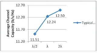
Figure 14 shows the average channel capacity of the typical MIMO system by changing the do. The value was increased 11.51 b/s/Hz to 12.50 b/s/Hz. The signals
can be uncorrelated since used the spatial diversity in order to increase MIMO channel capacity.
Figure 14: Average Channel Capacity for Typical MIMO
System by changing the d
λ λ
λ λ
λ
λ Figure 14: Average Channel Capacity for
Typical MIMO System by changing the do Based on the theoretical, the MIMO system that implemented polarization diversity has a potential in order to increase the channel capacity. Table 1 shows the average channel capacity of the typical MIMO system with polarization diversity as the do was λ and ro was 15λ. The coniguration C, I and N were having a inest average channel capacity compared to the typical MIMO system. The assortment of those conigurations was upon the comparison between the typical MIMO systems in terms of average channel capacity [23].
Based on Table 1, coniguration C and N has a beter average channel capacity compared to the typical MIMO system which the diference was 0.03 b/s/Hz and 0.09 b/s/Hz irrespectively. However, coniguration I show a lower average channel capacity compared to the typical MIMO system which the diference value of decrement was 0.06 b/s/Hz. In [24], the results show the channel capacity for system with polarization diversity has atained 21.3 b/s/Hz for without relector in the measurement setup and recently the value of coniguration C, I and N were below of that level [23].
to the degradation of the average channel capacity.
Table 1 Comparison of Average Channel Capacity between the Typical MIMO System and MIMO System with Polarization Diversity
since rsity technique.
was λ was 15λ.
system
e channel capacity of value is e signals can be rder to
λ λ
Polarization Diversity
Antenna Configuration Average Channel Capacity (b/s/Hz)
Typical MIMO System 12.24
C 12.27
I 12.18
N 12.33
λ λ
λ
λ
By referring to [23], coniguration G with polarization diversity at the receiver has a higher average channel capacity compared to the typical MIMO system at the distance was 96λ with antenna spacing λ. The average channel capacity for coniguration G was 11.71 b/s/Hz and the diference with the typical MIMO system was 0.49 b/s/Hz. The used of polarization diversity can reduce the mismatch losses at the receiver side. The mismatch losses happen because the signals that impinge on the surface of the physical path might change the polarity of the signals. The polarization diversity technique was used in order to increase the probability at the receiver side.
vIII. ConClUsIon
For the typical MIMO system that implemented the polarization diversity can improve the channel capacity. The average channel capacity also afected due to changing the antenna spacing. For example at the distance of 96λ, coniguration G with the polarization at receiver with antenna spacing λ has surpassed the average channel capacity of the typical MIMO system. The channel capacity was increase when the spacing between antennas increases. Most of the conigurations with polarization diversity show increment in channel capacity. However, the highest channel capacity was achieved when polarization diversity was applied at receiver side.
referenCes
[1] G.J. Foschini and M.J. Gans, “On Limits of Wireless Communication in a Fading Environment”, Wireless Personal Communications, vol. 6, pp.311-335,1998
[2] I. Emre Telatar, “Capacity of multi-antenna Gaussian Channels”, European transactions on telecommunications, vol. 10, no. 6, pp. 585-595, Nov./Dec 1999
[3] P. Stavroulakis “Interference Analysis
And Reduction For Wireless System”,
page 48, 2003
[4] K. Yu and Björn Otersten, “Models
for MIMO Propagation Channels,
A Review”, in Wiely Journal on
Wireless Communications and Mobile Computing Special Issue on Adaptive Antennas and MIMO Systems, 2002-07-08
[5] A. Botonjiæ, “MIMO channel models”,
Diploma Thesis, Examensarbete utfört i Elektronikdesign vid Linköpings Tekniska Högskola, Campus Norrköping,
[6] M.A Jensen, J.W Wallace (2004). A
Review of Antennas and Propagation
for MIMO Wireless Communications. IEEE Transaction on Antennas and Propagation pp. 2810 – 2824.
[7] T. Duman, M., Ghrayeb, Ali (2007). Coding For MIMO Communication Systems, England: John Wiley & Sons Ltd.
[8] V.R. Anreddy, M.A. Ingram, (2006). Capacity of Measured Ricean and Rayleigh Indoor MIMO Channels
at 2.4 GHz with Polarization and Spatial Diversity. IEEE Wireless Communication and Networking
Conference, 2006 (Anreddy, V. R &
Ingram, M. A.), pp. 946 -951
[9] J.P. Kermoal, et. al. (2002b). A Stochastic MIMO Radio Channel Model with Experimental Validation. IEEE Journal
on Selected Areas in Communications, pp. 1211 – 1226.
Propagation Society International Symposium, pp. 5335 – 5338.
[11] J. Hamalainen, et.al. (2005). Analysis and Measurement for Indoor Polarization MIMO in 5.25 GHz Band. IEEE 61st Vehicular Technology Conference, 2005, pp. 252 – 256, vol. 1.
[12] Pei-Yuan Qin et.al. (2010). Efect of Antenna Polarization Diversity on MIMO System Capacity. IEEE Antennas and Wireless Propagation
Leters, pp. 1092 – 1095
[13] J.M. Vella, S. Zammit, (2010), Performance Imprvement of Long Distance MIMO Links Using Cross Polarized Antennas. 15th IEEE Mediterranean Electrotechnical Conference 2010, pp. 1287 – 1292.
[14] Hsuch-Jyh Li & Chia-Hao Yu (2003).
Correlation Properties and Capacity of Antenna Polarization Combinations for
MIMO Radio Channel. IEEE Antennas
and Propagation Society International Symposium, 2003, pp. 503 – 506, vol. 2 [15] Xiaoyu Wang et.al. (2010). Measurement
on 2.3 GHz Wideband Indoor MIMO Channel Based On Dual Polarization Antennas. International Conference on Microwave and Millimeter Wave Technology (ICMMT), 2010, pp. 1805 – 1808
[16] Shahab Sanayei and Aria Nosratinia, “Antenna Selection in MIMO Systems”, Adaptive antennas and MIMO system for wireless communications. IEEE
Communications Magazine • October
2004
[17] Jean-Philippe Kermoal (2002).
Measurement, Modelling and Performance Evaluation of the MIMO
Radio Channel. Phd Thesis, Aalborg
University, 2002
[18] Richard Jaramillo E, Oscar Fernandez and Rafael P. Torres, “ Empirical Analysis of 2x2 MIMO channel in
Outdoor-Indoor Scenarios for BFWA Applications”, IEEE Antennas and Propagation Magazine, Vol. 48, No.6, December 2006
[19] Theodore S. Rappaport , ‘Wireless
communications (principle and Practice)’, Second Edition, Prentice Hall of India, 2007
[20] J. G. Proakis, 2001 ‘Digital
Communication’, Fourth Edition, McGraw-Hill Higher Education
[21] James R. Schot, 1997 “ Matrix Analysis for Statistics”, page 24, New York: John
Wiley & Sons.
[22] M.F.A. Kadir, M.Z.A. Abd. Aziz, M.K. Suaidi, M.R. Ahmad, Z. Daud, M.K.A. Rahim, “MIMO Beamforming Network
Having Polarization Diversity” 3rd European Conference on Antenna & Propagation 2009 (EuCAP2009), pp. 1743 – 1747.
[23] M.F.A. Kadir, M.K. Suaidi, M.Z.A. Abd
Aziz, “MIMO Beamforming Network Having Polarization Diversity” MIMO Systems: Theory and Application, InTech, ISBN: 978-953-307-245-6, pp: 415-420.
[24] H. Hirayama, et.al. (2007). An
Experimental Consideration on Spatial
and Minimum Eigenvalue for MIMO System Using Polarization. The Second European Confereance on Antennas and Propagation, 2007, pp 1 – 5 [25] Leilei Liu, Wei Hong ,“ Characterization
of line-of-sight MIMO channel for ixed
wireless Communications.”2007 [26] Andrea Goldsmith, Ali Jafar, Nihar
Jindal, Sriram Vishwanath, “ Capacity limits of MIMO channels”, IEEE journal on selected Areas in communications, Vol. 21, No.5, June 2003
[27] C. Pereira, Y.Chartois, Y. Pousset, R. Vauzelle, “ Impact Of Indoor
Environtment Modelling on MIMO Channel Characterization,” Proceedings of the 9th European Conference on Wireless technology,
Manchester UK [Sept. 2006].
[28] Wallace J., Jensen M., “mutual coupling in mimo wireless systems: a rigorous network theory analysis”, IEE Trans. Wireless Communication, 2004, pp.1130-1134.
[29] Claude Oestges “ Validity of the
Kronecker Model For MIMO