Sensitivity Analysis of a Two-Dimensional Probabilistic Risk
Assessment Model Using Analysis of Variance
Amirhossein Mokhtari
1and H. Christopher Frey
1∗
This article demonstrates application of sensitivity analysis to risk assessment models with two-dimensional probabilistic frameworks that distinguish between variability and uncertainty. A microbial food safety process risk (MFSPR) model is used as a test bed. The process of iden-tifying key controllable inputs and key sources of uncertainty using sensitivity analysis is challenged by typical characteristics of MFSPR models such as nonlinearity, thresholds, inter-actions, and categorical inputs. Among many available sensitivity analysis methods, analysis of variance (ANOVA) is evaluated in comparison to commonly used methods based on cor-relation coefficients. In a two-dimensional risk model, the identification of key controllable inputs that can be prioritized with respect to risk management is confounded by uncertainty. However, as shown here, ANOVA provided robust insights regarding controllable inputs most likely to lead to effective risk reduction despite uncertainty. ANOVA appropriately selected the top six important inputs, while correlation-based methods provided misleading insights. Bootstrap simulation is used to quantify uncertainty in ranks of inputs due to sampling error. For the selected sample size, differences inF values of 60% or more were associated with clear differences in rank order between inputs. Sensitivity analysis results identified inputs re-lated to the storage of ground beef servings at home as the most important. Risk management recommendations are suggested in the form of a consumer advisory for better handling and storage practices.
KEY WORDS:Microbial food safety process risk models; sensitivity analysis; two-dimensional proba-bilistic framework; uncertainty; variability
1. INTRODUCTION
This article demonstrates the application of sensitivity analysis to risk assessment models with two-dimensional probabilistic frameworks that distin-guish between variability and uncertainty. A micro-bial food safety process risk (MFSPR) model is used as a test bed. Although sensitivity analysis has been
1Department of Civil, Construction, and Environmental Engineer-ing, North Carolina State University, Raleigh, NC 27695-7908, USA.
∗Address correspondence to H. C. Frey, Department of Civil, Construction, and Environmental Engineering, North Carolina State University, Raleigh, NC 27695-7908, USA; tel: 919-515-1155; fax: 919-515-7908; [email protected].
applied to two-dimensional probabilistic frameworks in other scientific disciplines,(1,2)we believe this is the
first such systematic application to MFSPR models. Particular attention is given here to distinguishing be-tween variability and uncertainty in sensitivity analy-sis and its implication in providing more robust results and confidence in insights regarding key model inputs. The process of identifying key controllable inputs and key sources of uncertainty using sensitivity anal-ysis is challenged by typical characteristics of MFSPR models such as nonlinearity, thresholds, interactions, and categorical inputs.(3) Commonly used
sensitiv-ity analysis methods, such as correlation analysis, can be misleading when applied to complex MFSPR models.
Key methodological questions addressed in-clude: How does uncertainty in model inputs af-fect the ranking of key sources of variability? Does comingling variability and uncertainty into a single dimension provide different insight regarding key model inputs than two-dimensional simulation? How can one discriminate the importance between closely ranked inputs? What are the limitations of commonly used sensitivity analysis methods when applied to MFSPR models? What are the implications of sen-sitivity analysis for refinement of the analysis and for risk management?
Food safety risk assessment modeling is dis-cussed. Motivations for sensitivity analysis of MFSPR models are explained. The rationale for focusing on a selected sensitivity analysis method and an MFSPR model as a test bed is given.
1.1. Food Safety Risk Assessment Modeling
In the field of food safety, quantitative risk assess-ment is widely used to provide insight with respect to risk management strategies.(4,5) There has been
increasing development and use of MFSPR models for risk assessment of food-borne diseases.(6)
Exam-ples includeSalmonellain eggs,(7)E. coli O157:H7in
ground beef,(8)Vibrio parahaemolyticsin raw
mollus-can shellfish,(9)andListeria monocytogenesin
ready-to-eat (RTE) foods.(10)
MFSPR models generally have probabilistic frameworks, are able to quantify uncertainties in the population risk, include many parameters and inputs that have uncertainty and/or variability, have complex or highly nonlinear interactions between inputs, have threshold or saturation points in the model response, and use different types of inputs (e.g., continuous ver-sus categorical). A threshold is a value in an input do-main below which a model output does not respond to changes in the input. Similarly, a saturation point is an input value above which the model output does not re-spond. Parameters and inputs of MFSPR models are generally quantified by using probability distributions that represent variability, uncertainty, or both. Vari-ability represents true heterogeneity in the population that cannot be further reduced. Uncertainty repre-sents lack of perfect knowledge and can be reduced by further measurements.(11–20)
1.2. Need for Sensitivity Analysis
Sensitivity analysis has long been recognized as a useful adjunct for model building(1,21) Sensitivity
analysis highlights the inputs that have the great-est influence on the results of a model; therefore, it provides useful insights for model builders and users.(22)Sensitivity analysis provides insight
regard-ing which model input contributes the most to un-certainty, variability, or both, for a particular model output. Knowledge of key sources of uncertainty is useful in prioritizing additional data collection or research.
Knowledge of key sources of variability is useful in identifying control measures. Sensitivity analysis is an aid in developing priorities for risk mitigation and management strategies. Sensitivity analysis can be used to prioritize potential critical control points (CCP) in MFSPR models and identify corresponding critical limits. CCPs are points, steps, or procedures in the process of bringing food from farm to the table at which direct control can be applied, and a food safety hazard can be prevented, eliminated, or reduced to an acceptable level.(23,24)A critical limit (CL) is a
cri-terion that must be met for each preventive measure associated with a CCP.
1.3. Selection of the Sensitivity Analysis Method and the MFSPR Model for the Case Studies
A sensitivity analysis method applicable to MF-SPR models should be able to: deal with simul-taneous variation in inputs; address specific model characteristics such as nonlinearity, interactions, and thresholds; handle alternative input types (contin-uous versus categorical); discriminate among sen-sitive inputs; and provide quantitative measures of sensitivity.(3) A detailed comparison of the
capabili-ties of many sensitivity analysis methods with regard to these characteristics is given elsewhere.(25,26) A
key conclusion was that methods conventionally used for sensitivity analysis and available in commercial statistical software packages (e.g., correlation anal-ysis) may not provide robust results when applied to MFSPR models. However, analysis of variance (ANOVA) was identified as a promising method that can deal with nonlinearity, interaction, thresholds, and both categorical and continuous inputs. Thus, ANOVA is selected for application to the case studies in this article. Other promising methods, such as cat-egorical and regression trees (CART), are discussed elsewhere.(25,26)
E. coli O157:H7 organisms are estimated to be re-sponsible for some 73,500 cases of infection, 2,150 hospitalizations, and 61 deaths in the United States each year.(27)The model has a two-dimensional
prob-abilistic framework and typical characteristics of MFSPR models.
2. MODEL
2.1. Overview of theE. coli O157:H7Food Safety
Process Risk Model
The U.S. Department of Agriculture conducted a farm-to-table risk assessment to evaluate the pub-lic health impact from E. coli O157:H7 in ground beef.(8)TheE. coli O157:H7risk assessment includes
hazard identification, exposure assessment, hazard characterization, and risk characterization steps. The exposure assessment step consists of three major modules: (1) production; (2) slaughter; and (3) prepa-ration. The preparation module consists of three parts: (1) growth estimation; (2) cooking effect; and (3) serving contamination. The exposure assessment is based upon a probabilistic approach for model-ing the prevalence and the concentration of the E. colipathogen in live cattle, carcasses, beef trim, and a single serving of cooked ground beef. The model is implemented in Microsoft Excel using @Risk as an add-in for defining probability distributions for inputs.
The E. coli model has a modular framework. Thus, each key activity is modeled in a separate mod-ule. For example, there are separate modules for estimation of infection of live cattle on farms and contamination of meat trimmings in slaughter plants. Each module may have inputs that are calculated based upon a predecessor module and its outputs may be input to a successor module. In some cases, the out-put of a module is binned into predefined intervals prior to transferring to successor module. For exam-ple, in the slaughter module the contaminant concen-tration in beef trimings is estimated as a continuous output, but subsequently is binned by 0.5 log10
incre-ments from 0 to 8 log10.(8) Each log10 increment in
contamination represents a 10-times increase in the contamination level. Because of binning, there is a loss of one-to-one correspondence between outputs of one module and the inputs of its predecessors. Therefore, binning is an obstacle to global sensitiv-ity analysis of the entire model. Creating one-to-one correspondence in this case would require
substan-tial restructuring and recoding of the model. Thus, ANOVA is applied to the individual modules.
2.2. Growth Estimation Part
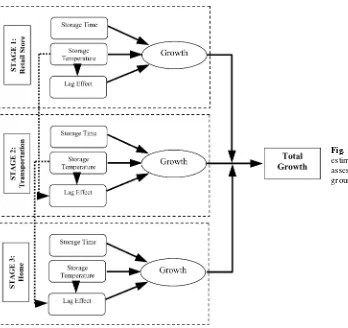
The growth estimation part in the preparation module is selected for the case studies (Fig. 1). This part has a two-dimensional probabilistic simulation framework. Storage temperature and storage time at retail (Stage 1), transportation (Stage 2), and home (Stage 3) influence the E. coli O157:H7 levels in ground beef servings. The output is the growth ofE. coli O157:H7organisms in ground beef servings prior to cooking.(8)
The log of growth for each stage is a function of storage temperature (T), lag period duration (LP), and generation time (GT). LP is the time that organ-isms take to become acclimated to a new environment before starting to multiply. GT is the interval from one point in the division cycle of an organism to the same point in the cycle one division later. The log of growth in Stage ‘i’ is calculated as:
Gi=log10
2LPiGTi−Ti. (1)
Growth is calculated in each stage only if stor-age temperature is greater than 45◦F, and hence a set of eight potential growth combinations that can occur in Stage 1 through 3 for a single ground beef serving is considered based on the probability that each serving is kept at a temperature above 45◦F at each stage. The lag period in Stages 2 and 3 are ad-justed based on the cumulative lag used in previous stages. At each stage, calculated growth is compared with the theoretic maximum density at refrigeration temperature and the smaller value is considered as the possible growth. Maximum density (MD) is the maximum possible number ofE. coli O157:H7 organ-isms at a specific storage temperature on a serving. More explanation of the modeling approach is given in FSIS.(8)
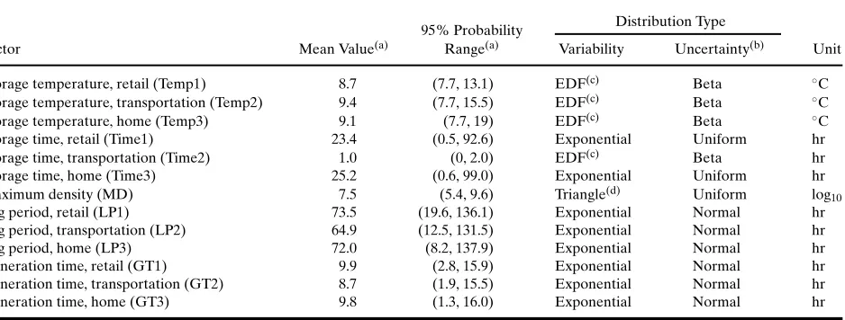
Table I summarizes 13 inputs, including their mean values and 95% probability ranges based on the sampled values of inputs in a comingled ysis of variability and uncertainty. Comingled anal-ysis of variability and uncertainty is explained in Section 3.4.2. Table I also gives the type of variability and uncertainty distributions for each input.(8)
Fig. 1.Schematic diagram of the growth estimation part of the farm-to-table risk assessment model forE. coli O157:H7in ground beef.
3. MATERIALS AND METHODS
3.1. Overview of ANOVA
ANOVA is a model-independent sensitivity anal-ysis method with no assumption regarding the func-tional relationship between the output and inputs and that makes simultaneous comparisons to deter-mine differences among the means of two or more groups on a variable. ANOVA assumes that the re-sponse at each value of the inputs is normally dis-tributed with the same variance.(28–32) Nonetheless,
ANOVA is generally robust to deviations from this assumption.(33,34)
An input is referred to as a “factor” and specific ranges of values for each factor are defined as factor “levels.” A “treatment” is a specific combination of levels for different factors. An output is referred to as a “response variable,” and a “contrast” is a linear com-bination of two or more factor-level means.(35)For
ex-ample, a contrast can be used to evaluate the change in the mean growth of pathogens when the storage temperature varies between high and low levels for a specific storage time. Contrasts typically provide
in-sight regarding specific model characteristics such as threshold and saturation points.
Categorical factors are easily treated as levels. Continuous factors can be partitioned to mutually ex-clusive and exhaustive subintervals in order to cre-ate levels.(36) The optimal definition of levels for a
continuous factor is often a matter of judgment and some experimentation may be required to determine an appropriate division.(25,36)
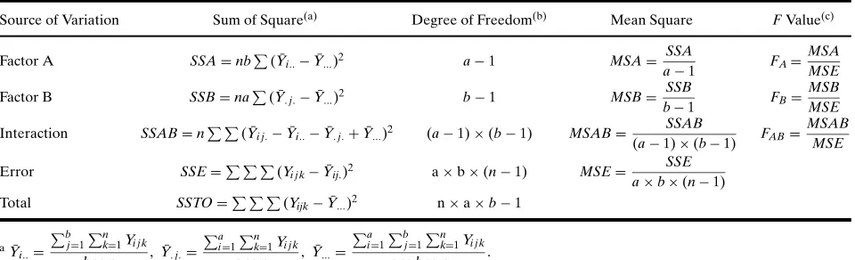
ANOVA is used to analyze the effects of the fac-tors on the response variable. ANOVA can decom-pose the response variable (Y) into an overall mean (µ), main factor effects, interaction effects, and an er-ror term (ε). AVOVA provides estimates of overall mean and factor main and interaction effects. For ex-ample, for a two-way ANOVA:(35)
Yi,j,k=µ+αi+βj+(α×β)i,j+εi,j,k, (2)
Table I. Input Variables and Corresponding Mean Values, 95% Probability Ranges, and Distribution Types in the Growth Estimation Part of theE. coliModel(8)
Distribution Type 95% Probability
Factor Mean Value(a) Range(a) Variability Uncertainty(b) Unit
Storage temperature, retail (Temp1) 8.7 (7.7, 13.1) EDF(c) Beta ◦C
Storage temperature, transportation (Temp2) 9.4 (7.7, 15.5) EDF(c) Beta ◦C
Storage temperature, home (Temp3) 9.1 (7.7, 19) EDF(c) Beta ◦C
Storage time, retail (Time1) 23.4 (0.5, 92.6) Exponential Uniform hr
Storage time, transportation (Time2) 1.0 (0, 2.0) EDF(c) Beta hr
Storage time, home (Time3) 25.2 (0.6, 99.0) Exponential Uniform hr
Maximum density (MD) 7.5 (5.4, 9.6) Triangle(d) Uniform log
10
Lag period, retail (LP1) 73.5 (19.6, 136.1) Exponential Normal hr
Lag period, transportation (LP2) 64.9 (12.5, 131.5) Exponential Normal hr
Lag period, home (LP3) 72.0 (8.2, 137.9) Exponential Normal hr
Generation time, retail (GT1) 9.9 (2.8, 15.9) Exponential Normal hr
Generation time, transportation (GT2) 8.7 (1.9, 15.5) Exponential Normal hr
Generation time, home (GT3) 9.8 (1.3, 16.0) Exponential Normal hr
aValues are based on the comingled analysis of variability and uncertainty (see Section 3.4.2). bUncertainty distributions are defined for parameters of variability distributions.
cEmpirical distribution function (EDF) based on FSIS data.(8)Beta distribution is used to define the corresponding cumulative frequency
at each temperature as:
C Fi=BetaINV(α, β)
where,
i =Cumulative rank of data associated with a temperature.
CFi =Cumulative frequency at valueiof the empirical distribution.
BetaINV=Inverse of a beta distribution.
α =Parameterαof the beta distribution: i k=1nk.
β =Parameterβof the beta distribution: nT−ik=1nk+1.
ni =Number of available data at theith value of storage temperature.
nT =Total number of available survey data.
dUncertainty is defined for the most likely value of the triangular distribution.
the main effect of thejth level of FactorB, and the in-teraction effect between the two factors. If additional factors are involved in the analysis, the concept will be the same.
ANOVA uses theF-test to determine whether a statistically significant difference exists among mean responses for main effects or interactions between factors. TheF-test is used to test the significance of each main and interaction effect. For the example of Equation (2), the estimators ofFvalues for main and interaction effects are given in Table II.(35)The
rela-tive magnitude ofFvalues can be used to rank the fac-tors in sensitivity analysis.(37)The higher theFvalue,
the more sensitive the response variable is to the fac-tor. Therefore, factors with higherFvalues are given higher rankings.
The coefficient of determination, R2, is used to judge the adequacy of the ANOVA model.R2 mea-sures the proportionate reduction of total variation in the response variable (Y) associated with the use
of selected main and interaction effects of factors in the ANOVA model.(33–35) Although the F values
calculated for each effect indicate the statistical sig-nificance of corresponding effect, the coefficient of determination indicates whether the selected effects adequately capture variability in the output. Gen-erally, a high R2 value implies that results are not
compromised by incomplete specification of effects or by inappropriate definition of the levels for a fac-tor. When ANOVA is applied to two-dimensional simulations of variability and uncertainty, a CDF graph for R2 indicates uncertainty in the adequacy of the ANOVA model for multiple realizations of the model.
3.2. Correlation Coefficients
Table II. ANOVA Table for a Two-Factor Model
Source of Variation Sum of Square(a) Degree of Freedom(b) Mean Square FValue(c)
Factor A SSA=nb
ba=number of levels for Factor A; b=number of levels for Factor B; n=number of values for the response variable. c5% significance level is considered for statistically significantFvalues.
as a useful benchmark for comparison with ANOVA. The Pearson correlation coefficient (PCC), for in-stance, can be used to characterize the degree of linear relationship between the output values and sampled values of individual inputs. If the relationship between an input and an output is nonlinear but monotonic, Spearman correlation coefficients (SCC) provide bet-ter performance.(38–40) SCCs are based on ranks, not
sample values, of each input and output. Neither PCCs nor SCCs can provide insight regarding possible in-teraction effects between inputs. The magnitude of a PCC or SCC is typically used as a basis to rank order model inputs based on their influence on the output.
3.3. Top-Down Correlation for Comparison of Sensitivity Analysis Methods
When applying different sensitivity analysis methods to a case study, an important question is whether different techniques agree in their identifica-tion of important inputs. The so-called top-down cor-relation method is useful for this purpose. Details of the method are available elsewhere.(36,41)This method
gives greater weight to agreement or disagreement in rank ordering of the most important inputs and gives less weight to comparisons in ranks of inputs with low importance. Large positive values for the top-down correlation result indicate agreement between two sets of ranks for the most important inputs.
3.4. Probabilistic Analysis Scenarios
Two scenarios are introduced: (1) variability anal-ysis for different realizations of uncertainty; and (2)
comingled analysis of variability and uncertainty. Pro-cedures for application of sensitivity analysis to these scenarios and specific insights with respect to sensitiv-ity that can be obtained from each of these approaches are briefly discussed.
3.4.1. Variability Analysis for Different Uncertainty Realizations
In variability analysis for different uncertainty re-alizations, the objective of the analysis is to distinguish between variability and uncertainty in order to prop-erly distinguish between inherent differences in val-ues among members of a population versus lack of knowledge.(2,15,19)As illustrated in Fig. 2, the focus
of sensitivity analysis in this approach is to identify the key variability inputs for each realization of un-certainty.(1,2)A realization refers to one model
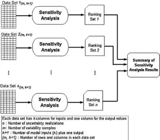
simu-lation based upon one randomly sampled uncertainty value for each probabilistic input. In this situation, sensitivity analysis provides insight regarding whether the identification of the key sources of variability is robust with respect to uncertainty. Each data set in Fig. 2 includes randomly generated values (e.g., m
values) from variability distributions of each model input for a given uncertainty realization and the cor-responding model output values. Sensitivity analysis is applied separately to each data set. Thus, for each realization, the key sources of variability, critical lim-its, or both, are identified. This process is repeated
Fig. 2.Case study scenario for application of sensitivity analysis to variability analysis for different uncertainty realizations of a model.
uncertainty realization of the model when the inputs are sorted according to their sensitivity indices. A rank of 1 is assigned to an input with the highest sensi-tivity index, and the largest numerical value of rank was assigned to the input with the least importance (i.e., lowest sensitivity index). For example, when us-ing ANOVA, for each uncertainty realization inputs are ranked based on the relative magnitude ofF val-ues, and hence, n ranks are assigned to each input, wheren represents the number of uncertainty real-izations of the model. For this probabilistic scenario, values of 100 and 650 were selected fornandm, re-spectively, based upon the storage limit in each Excel sheet.
To the extent that the sensitivity analyses yield similar results about the rank ordering of key in-puts regardless of uncertainty, an analyst or deci-sionmaker will have greater confidence that the re-sults of the analysis are robust to uncertainty. If the ranking of key inputs changes substantially from one realization of uncertainty to another, the iden-tification of key inputs would be uncertain. Addi-tional data collection or research may reduce this ambiguity.
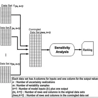
3.4.2. Comingled One-Dimensional Variability and Uncertainty Analysis
There may be situations in which it is either not necessary or perhaps not possible to distinguish be-tween variability and uncertainty. If either variability or uncertainty dominates the assessment, then it may not be necessary to distinguish between the two, nor is it necessary to separate the two if the focus is on a randomly selected individual. Furthermore, during the process of model building, an analyst may want to estimate the widest range of values that might be assigned to each model input for purposes of verify-ing the model and evaluatverify-ing the robustness of the model to large perturbations in its inputs. As a pre-liminary step in prioritizing data collection or the de-velopment of distributions for model inputs, an an-alyst may wish to assess the key sources of variation regardless of whether they represent variability or un-certainty. In some cases, an analyst may make a judg-ment that it is difficult to separate variability from uncertainty,(6) or that a two-dimensional
Fig. 3.Case study scenario for application of sensitivity analysis to the comingled variability and uncertainty analysis of a model.
based on a “one dimensional” comingling of vari-ability and uncertainty are compared to those from a “two-dimensional” simulation in which variability and uncertainty are distinguished. The latter is typi-cally preferred where possible and appropriate to the assessment objective.
Fig. 3 illustrates sensitivity analysis in the context of comingled variability and uncertainty. There is one data set generated for each of the uncertainty real-izations of the model. Each data set hasm rows of randomly generated samples from variability distri-butions and the corresponding output values. Prior to application of sensitivity analysis, these data sets are appended together to form a single data set with
n×mrows. Sensitivity analysis is then applied to the comingled data set and a set of rankings is obtained. For the comingled analysis in the growth estimation part values of 100 and 650 were selected fornandm, respectively.
4. RESULTS
This section presents results from application of ANOVA to each of the probabilistic scenarios defined in Section 3.4. For each probabilistic scenario, results from ANOVA are compared with results from
Pear-son and Spearman correlation analyses. Application of ANOVA to identify a saturation point in the model response and a methodology for quantifying ambigu-ity in ranks in a one-dimensional analysis is demon-strated. Ranking of the important factors based on ANOVA also is verified.
4.1. Application of ANOVA
Inputs in the growth estimation part are continu-ous, and hence must be partitioned into levels.(36)Frey et al.demonstrated three approaches for defining fac-tor levels for continuous inputs based on: (1) evenly spaced intervals; (2) evenly spaced percentiles; and (3) visual inspection of the cumulative distribution function (CDF) for each input.(25) For the first
ap-proach, each input domain is classified into equal ranges. For the second approach, the CDF of the gen-erated values for an input in a probabilistic simula-tion is used for defining factor levels at evenly spaced percentiles. For the third approach, boundaries for each factor level are defined corresponding to per-centiles of the CDF that are associated with a sub-stantial change in the slope.
Table III.Levels Defined for Factors in the Growth Estimation Part of theE.
coliModel
Number Levels and Corresponding
Factor(a) of Levels Percentiles(b)
Temp1 5 7.5–11, 11–14.5, 14.5–18, 18–21.5,>21.5(c)
Temp2 3 7.5–13.5, 13.5–19.5,>19.5(c)
Temp3 5 7.5–11, 11–14.5, 14.5–18, 18–21.5,>21.5(c)
Time1 12 0–24, 24–48,. . ., 264–288,>288(c)
Time2 2 0–3.5,>3.5(c)
Time3 12 0–24, 24–48,. . ., 264–288,>288(c)
MD 3 {<6.5,6.5–8.5,>8.5} {20th, 80th}Percentiles
LP1 4 {<50, 50–65, 65–95,>95} {20th, 50th, 80th}Percentiles LP2 4 {<35, 35–55, 55–90,>90} {20th, 50th, 80th}Percentiles LP3 4 {<45, 45–65, 65–95,>95} {20th, 50th, 80th}Percentiles GT1 4 {<7, 7–9.5, 9.5–12.5,>12.5} {20th, 50th, 80th}Percentiles GT2 4 {<4.5, 4.5–8, 8–12,>12} {20th, 50th, 80th}Percentiles GT3 4 {<6.5, 6.5–9.5, 9.5–13,>13} {20th, 50th, 80th}Percentiles
aThe abbreviations used for factors in this table are the same as those defined in Table I. bThe ranges that define each factor level and the percentiles of the CDF corresponding to the
breakpoint between factor levels are given.
cFor this factor equal intervals are used as levels.
the power of statistical tests.(42)There is a tradeoff
be-tween selecting a larger number of factor levels, which can produce more highly resolved insights regarding sensitivity, and getting statistically significant results. There is also a tradeoff between the desired number of iterations (e.g., in a Monte Carlo simulation) that are used to populate factor levels and the computa-tional time.
Table III summarizes the levels defined for factors in the case studies. These levels are used in both proba-bilistic scenarios. Levels are mostly defined based on visual inspection of the CDF for each factor. Each CDF is prepared based on the generated values for a factor in the comingled analysis of variability and un-certainty, since this probabilistic approach gives the widest range of variation for each factor. For storage times at Stages 1 and 3, levels are defined at equal intervals.
4.2. Variability Analysis for Different Uncertainty Realizations
4.2.1. Rankings Based on ANOVA
Table IV summarizes the results from variability analysis for different uncertainty realizations. Mean, minimum, and maximum estimatedFvalues from all uncertainty realizations for each factor are given. The percentage of the uncertainty realizations that pro-duced a statistically significantFvalue for each factor is quantified. The mean rank and the range of ranks
are presented. For each uncertainty realization, in-teractions between storage temperature and storage time at all three stages are evaluated.
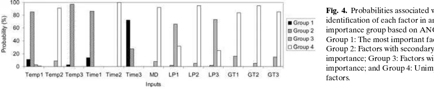
The factors were classified into four groups based on their ranks in uncertainty realizations: (1) Group 1: the most important factor with rank 1; (2) Group 2: factors with secondary importance with ranks between 2 and 4; (3) Group 3: factors with mi-nor importance with ranks 5 and 6; and (4) Group 4: factors that were unimportant with ranks between 7 and 13. Factors in the latter group typically were not identified as statistically significant in most of un-certainty realizations. Because the rankings of fac-tors typically varied among uncertainty realizations, often a given factor might be assigned to different groups in different uncertainty realizations. However, there was typically a group to which each factor was most frequently assigned. The probabilities associ-ated with assignment of a given factor to each of the four groups were estimated based on the num-ber of times the factor was assigned to the selected group divided by the total number of uncertainty realizations.
Table IV.Summary of the ANOVA Results for Two-Dimensional Variability
Simulation for Different Uncertainty Realizations
[min, max] Mean Range of
Factor(a) MeanFValue Range ofFvalues(b) Frequency(c) Rank(d) Rank
Temp1 103.0 (2.0, 1233.0) 98 3.1 1–8
Temp2 1.0 (0.0, 14.6) 10 11.2 5–13
Temp3 118.9 (16.9, 689.3) 100 2.7 1–4
Time1 99.0 (6.8, 495.4) 100 2.8 1–4
Time2 0.3 (0.1, 2.7) 0 12.3 10–13
Time3 188.4 (31.6, 1448.8) 100 1.5 1–4
MD 1.1 (0.1, 5.9) 6 11.7 5–13
LP1 4.8 (0.6, 18.1) 77 6.2 4–11
LP2 1.1 (0.1, 7.4) 6 11.8 5–12
LP3 4.6 (0.3, 14.4) 87 6.0 4–12
GT1 2.0 (0.1, 47.3) 14 11.0 5–13
GT2 1.0 (0.1, 4.4) 10 11.5 5–13
GT3 1.4 (0.1, 9.4) 11 11.1 5–13
Time1×Temp1 66.2 (10.5, 339.8) 100
Time2×Temp2 0.7 (0.1, 4.5) 2
Time3×Temp3 122.8 (46.4, 839.9) 100
aThe abbreviations used for factors in this table are the same as those defined in Table I. bRepresents minimum and maximumFvalues estimated for each factor in 100 uncertainty
realizations.
cThe percentage of the uncertainty realizations for which the F values were statistically
significant.
dArithmetic average of 100 ranks for each factor.
with mean ranks of 6.0 and 6.2, respectively. Group 4 contained seven factors—GT1, GT3, GT2, Temp2, LP2, MD,andTime2with mean ranks between 11.0 and 12.3.
The interaction effect between storage tempera-ture and storage time at Stage 2 was unimportant. The interaction effect between storage time and storage temperature at home had higher importance than in-teraction between similar factors at retail stores. The meanFvalues estimated for these two interaction ef-fects differed by a ratio of approximately 2. Although the interaction effects were not considered in the over-all ranking in Table IV, their relative importance can be compared with main effects using their meanF val-ues, similar to an approach presented by Roseet al.(43)
Fig. 4.Probabilities associated with identification of each factor in an importance group based on ANOVA. Group 1: The most important factor; Group 2: Factors with secondary importance; Group 3: Factors with minor importance; and Group 4: Unimportant factors.
Factors contributing to the two statistically significant interaction effects had relatively large mean F val-ues and were categorized in the first two importance groups. The interaction effect between Time3 and
Temp3had a meanFvalue approximately the same as that ofTemp3. Thus, the interaction had comparable importance withTemp3.
4.2.2. Diagnostic Check for Results Based on ANOVA
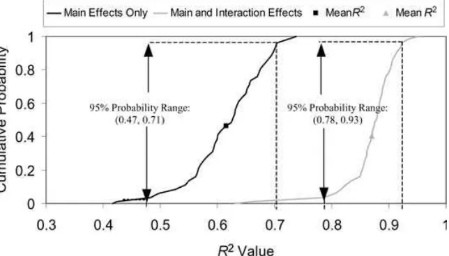
Fig. 5.Cumulative probability distribution ofR2values in the two-dimensional analysis for a model including only main effects and a model including both main and interaction effects.
variable,Y, captured by the ANOVA model at each uncertainty realization. Two ANOVA models were considered based on: (1) only the main effects of all factors; and (2) the main effects of all factors along with interaction effects given in Table IV. The com-parison of the two cases provided insight with respect to improvement in the amount of the variability in the response captured by the ANOVA model when interactions were also considered.
Fig. 5 shows CDF graphs forR2values estimated
in 100 uncertainty realizations for the two ANOVA models. For an ANOVA model based only on the main effects, the 95% probability range ofR2values was between 0.47 and 0.71 with a mean value of 0.62. For an ANOVA model based on all of the main effects and selected interactions, the 95% probability range ofR2values was between 0.78 and 0.93 with a mean value of 0.87. Therefore, interaction effects between storage time and storage temperature in Stages 1 to 3 accounted for an average of 25% of the total vari-ability in the response variable. Because the ANOVA model with interaction terms accounted for a substan-tial amount of variability in the response, ranks based on theFvalues were deemed to be reliable.
4.2.3. Rankings Based on Pearson and Spearman Correlation Analyses
Pearson and Spearman correlation analyses were selected as conventional sensitivity analysis methods for comparison with ANOVA. Inputs were ranked based on the absolute values of statistically significant correlation coefficients with a significance level of 5%. Table V summarizes mean ranks, range of ranks, and the percentage of the uncertainty realizations that
produced a statistically significant correlation coef-ficient. These methods are not able to provide insight with respect to interactions between inputs. Similar to ANOVA results, inputs were grouped into four cate-gories based on their ranks.
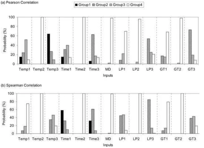
The probabilities associated with selection of in-puts in each of the four importance groups are shown in Fig. 6. Inputs within a given group were typically dif-ferent from those based on the ANOVA results. Some inputs implied to be sensitive based on PCC and SCC results (e.g.,GT3andLP3) were not found to be sen-sitive based on ANOVA. Among statistically signifi-cant inputs, there was not a clear agreement between the ranks based on the ANOVA results and those from Pearson and Spearman correlation analyses. For example, while ANOVA selectedTime3as the most important factor,Temp3andTime1were selected as the most important inputs based on PCC and SCC, respectively.
Table VI presents the results from top-down correlation analysis for pairwise compar-isons of the results for PCC, SCC, and ANOVA, based on the two-dimensional probabilistic sim-ulation. For each uncertainty realization, ranks based on each pairwise combination of sensitiv-ity analysis methods were compared and the top-down correlation coefficients between ranks were calculated.
Table V.Summary of Pearson and Spearman Correlation Analyses Results
for Two-Dimensional Variability Simulation for Different Uncertainty
Realizations Pearson Correlation Analysis Spearman Correlation Analysis
Mean Range Mean Range of
Inputs(a) Frequency(b) Rank of Rank Frequency(c) Rank Rank
Temp1 93 4.4 1–12 97 6.9 3–12
Temp2 2 11.0 8–13 7 11.1 9–13
Temp3 100 1.8 1–6 100 5.1 3–8
Time1 91 4.4 1–10 100 1.7 1–5
Time2 2 10.7 7–13 6 10.9 7–13
Time3 100 3.8 1–8 100 2.0 1–6
MD 3 10.8 9–13 1 10.9 9–13
LP1 81 7.0 3–13 99 4.8 2–8
LP2 5 10.5 6–13 8 10.8 7–13
LP3 99 4.9 2–111 100 3.3 2–8
GT1 80 6.8 2–13 94 7.3 4–12
GT2 1 11.3 9–13 4 11.2 10–13
GT3 99 3.7 2–9 100 5.2 3–8
aThe abbreviations used for factors in this table are the same as those defined in Table I. bThe percentage of the uncertainty realizations for which the F values were statistically
significant.
cThe percentage of uncertainty realizations for which coefficients were statistically significant.
realizations in which the top-down correlation was greater than 0.8.
4.2.4. Summary of the Results for the Variability Analysis for Different Uncertainty Realizations
The key insights and findings based on analysis of variability for different uncertainty realizations in-clude:
Fig. 6.Probabilities associated with identification of each input in an importance group based on: (a) Pearson correlation; and (b) Spearman
correlation. Group 1: The most important input; Group 2: Inputs with secondary importance; Group 3: Inputs with minor importance; and Group 4: Unimportant inputs.
r
There is a substantial range of uncertainty inthe relative importance of inputs due to uncer-tainty in the probability distribution of inputs.
r
Although the ranking of inputs varied amongTable VI. Top-Down Correlation Matrix for Input Rankings with Different Sensitivity Analysis Methods
Top-Down Correlation Results(b)
Method(a) ANOVA PCA SCA
−0.04 0.10
ANOVA (−0.34, 0.36) (−0.28, 0.45)
0 0
PCA 0.59 (0.26, 0.87)
11
aANOVA: analysis of variance; PCA: Pearson correlation analysis;
SCA: Spearman correlation analysis.
bFor each pair of methods, mean, 95% probability range, and
number of times that the top-down correlation coefficient was larger than 0.8 in uncertainty realizations are given.
r
The results based on Pearson and Spearmancorrelation typically were different compared to those based on ANOVA with respect to identification of key important inputs. How-ever, the two correlation-based methods iden-tified similar results with respect to unimpor-tant inputs compared to ANOVA.
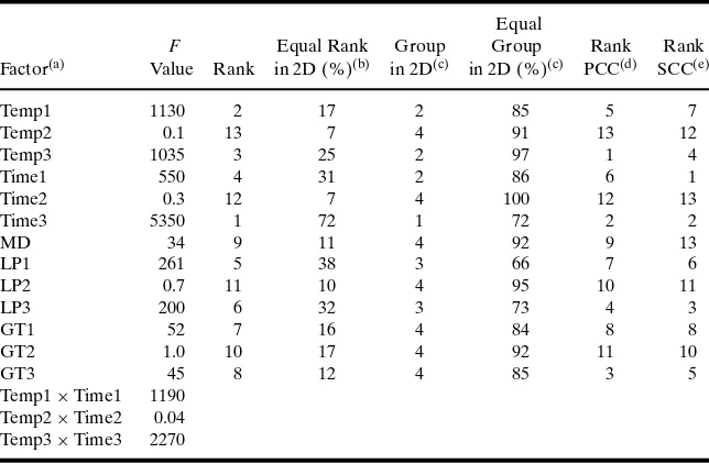
Table VII.Summary of the ANOVA Results for Comingled Analysis of Variability and Uncertainty (R2=0.82)
Equal
F Equal Rank Group Group Rank Rank
Factor(a) Value Rank in 2D (%)(b) in 2D(c) in 2D (%)(c) PCC(d) SCC(e)
Temp1 1130 2 17 2 85 5 7
Temp2 0.1 13 7 4 91 13 12
Temp3 1035 3 25 2 97 1 4
Time1 550 4 31 2 86 6 1
Time2 0.3 12 7 4 100 12 13
Time3 5350 1 72 1 72 2 2
MD 34 9 11 4 92 9 13
LP1 261 5 38 3 66 7 6
LP2 0.7 11 10 4 95 10 11
LP3 200 6 32 3 73 4 3
GT1 52 7 16 4 84 8 8
GT2 1.0 10 17 4 92 11 10
GT3 45 8 12 4 85 3 5
Temp1×Time1 1190 Temp2×Time2 0.04 Temp3×Time3 2270
aThe abbreviations used for factors in this table are the same as those defined in Table I. bPercent of times that rank in the comingled analysis equals the rank based on 2D analysis. cGroup 1: most important input (i.e., rank 1); Group 2: secondary importance inputs (i.e.,
ranks between 2 and 4); Group 3: minor importance inputs (i.e., ranks between 5 and 6); Group 4: unimportant inputs (i.e., ranks between 7 and 13).
dRank based on Pearson correlation analysis. eRank based on Spearman correlation analysis.
4.3. Comingled Analysis of Variability and Uncertainty
4.3.1. Rankings based on ANOVA
Table VII summarizes results when variability and uncertainty were comingled into one dimension. The main effects of all factors and interaction effects between storage temperature and storage time at all three stages were evaluated. For each factor the num-ber of times that the comingled analysis provided the same ranking as the two-dimensional sensitivity analysis was quantified.
Typically, the F values based on the comin-gled analysis of variability and uncertainty were sub-stantially larger than those for the two-dimensional analysis. This is in large part because there was a sub-stantially larger simulation sample size for the levels of each factor, which in turn reduces the sampling error.
Temp1 had a rank of 2 in the comingled analysis. However,Temp1 had a rank of 2 in only 17 out of 100 uncertainty realizations of the model in the two-dimensional analysis.
In contrast, when grouping factors with compara-ble importance, there was typically high concordance between the two probabilistic approaches. For exam-ple, Temp1 was assigned to Group 2 based on the comingled analysis. Similarly, in 85 out of 100 uncer-tainty realizations,Temp1had a rank between 2 and 4, and hence was assigned to the same importance group.
There was a statistically significant interaction be-tween storage time and storage temperature at Stages 1 and 3. The relative magnitude ofFvalues indicated that the interaction effect between these two factors at Stage 3 had higher importance. Similar to the two-dimensional analysis, there was no statistically signif-icant interaction between storage time and storage temperature at Stage 2.
4.3.2. Rankings Based on Pearson and Spearman Correlation Analyses
Rankings based on Pearson and Spearman corre-lation analyses typically were different from ANOVA results, except for inputs related to Stage 2. All three methods identified no statistically significant effects for inputs related to Stage 2. Groups of inputs with comparable importance based on Pearson and Spear-man correlation analysis results were different from those identified by ANOVA. For example, the most important inputs based on Pearson and Spearman correlation analysis wereTemp3andTime1, respec-tively, which were different fromTime3selected by ANOVA. Similarly, there was lack of agreement for inputs selected in secondary and minor importance groups based on these methods.
4.3.3. Quantification of Sampling Distribution of F Values
When performing one-dimensional probabilistic analysis, a key question is regarding how large the differences inF values between two factors must be in order to clearly discriminate their importance. A method for answering this question is illustrated. The range of sampling distributions ofFvalues provides insight regarding how large the ratio of twoF values must be in order for the ranks of the corresponding factors to be substantially different.
Empirical bootstrap simulation was used to gen-erate sampling distributions of uncertainty for F
values.(44)In the empirical bootstrap approach, an
al-ternative randomized version of the original Monte Carlo simulation was obtained by sampling with replacement from the original set of random values. ANOVA was applied to each of the bootstrap samples to produce a distribution ofFvalues. Summary of the results from 200 bootstrap simulations are given in Table VIII. The summary table is comprised of mean
Fvalues, 95% probability range ofFvalues, and coef-ficients of variation. The percentage of the bootstrap simulations that produced a statistically significantF
value with a significance level of 5% for each factor is quantified. The arithmetic mean of 200 ranks and the range of ranks for each factor also are quantified.
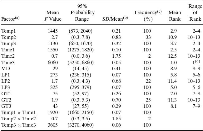
There was a substantial range of uncertainty as-sociated with the estimates ofFvalue. For example,
Temp1was estimated to have a mean rank of 2.9. The
F value for this factor had a mean of 1445 and 95% probability range of 873–2040, or approximately plus or minus 40% of the mean.Temp3had a mean rank of 3.7, a meanFvalue of 1130, and a 95%probability range of 650–1670, or approximately plus or minus 48%. The sampling distributions of theF values for these two factors did not have statistically significant correlation. Thus, the overlap in the confidence in-tervals of Temp1 and Temp3 indicated a possibility that the rank order between these two factors could reverse, even though on average theFvalue forTime1
was larger than that forTemp3by a factor of 1.3. This reversal in ranks happened in 32% of bootstrap sim-ulations. In contrast,Temp3had a statistically signif-icantly larger F value than the factor with the fifth highest average rank, which wasLP3. The 95% prob-ability ranges forFvalues of these two factors did not overlap. Therefore, although there was some ambigu-ity regarding which of the factors might be the third most important, it was clear thatTemp1,andTemp3
were more important thanLP3.
Table VIII.Summary of the ANOVA Results for 200 Bootstrap Simulations
forFValue Statistics
95% Range
Mean Probability Frequency(c) Mean of
Factor(a) FValue Range SD/Mean(b) (%) Rank Rank
Temp1 1445 (873, 2040) 0.21 100 2.9 2–4
Temp2 2.7 (0.3, 7.8) 0.83 33 10.9 10–13
Temp3 1130 (650, 1670) 0.32 100 3.7 2–4
Time1 1550 (1275, 1820) 0.10 100 2.5 2–4
Time2 0.7 (0.0, 3.6) 1.75 2 12.5 10–13
Time3 6060 (5250, 6860) 0.05 100 1.0 1(d)
MD 29 (14, 45) 0.41 100 8.9 8–9
LP1 273 (236, 315) 0.07 100 5.8 5–6
LP2 1.7 (0.3, 4.3) 0.68 22 11.4 10–13
LP3 325 (295, 379) 0.07 100 5.0 5–6
GT1 75 (52, 97) 0.26 100 7.0 7–8
GT2 1.9 (0.3, 5.3) 0.70 25 11.3 10–13
GT3 43 (27, 55) 0.29 100 8.1 7–9
Temp1×Time1 1920 (1660, 2150) 0.07 100
Temp2×Time2 0.7 (0.3, 3.5) 1.85 2
Temp3×Time3 3605 (3270, 4060) 0.06 100
aThe abbreviations used for factors in this table are the same as those defined in Table I. bThe ratio of standard deviation (SD) to meanFvalues for each factor (also referred to as
coefficient of variation).
cThe percentage of the bootstrap simulations for which the F values were statistically
significant.
dTime3consistently had rank 1 in bootstrap simulations.
was specific to the example provided here and should not be used to make general quantitative judgments regarding differences betweenFvalues obtained with different sample sizes or models. However, the tech-nique used here can be applied to other case studies. The case study results suggest that the model output has similar sensitivity to two or more factors if they have similarFvalues.
4.3.4. Summary of the Results for the Comingled Analysis of Variability and Uncertainty
Key insights and findings based on the comingled analysis of variability and uncertainty include:
r
Comingled analysis typically provideddiffer-ent results with respect to rank of impor-tant inputs compared to the two-dimensional analysis. However, both probabilistic ap-proaches identified similar groups of inputs with comparable importance.
r
Similar to the two-dimensional case, the twocorrelation-based methods failed to provide the same insights with respect to identifica-tion of the most important inputs compared to ANOVA.
r
In order to have statistically significantlydiffer-ent ranks, the two factors should haveFvalues that differ at least by 60% for the conditions of the case study.
4.4. Identifying Special Model Characteristics Using ANOVA
Table IX.Evaluation of ANOVA Contrasts for the Growth Estimation Regarding the Interactions Between Storage Temperature and Storage Time
at Stage 3
Contrast Estimate(a) FValue Pr>F Significant(b)
T [7.5–11◦C], Time 1st and 2nd days 0.005 112 <0.0001 Yes T [7.5–11◦C], Time 2nd and 3rd days 0.026 1280 <0.0001 Yes T [7.5–11◦C], Time 3rd and 4th days 0.049 1720 <0.0001 Yes T [7.5–11◦C], Time 4th and 5th days 0.069 1280 <0.0001 Yes T [7.5–11◦C], Time 5th and 6th days 0.074 610 <0.0001 Yes T [7.5–11◦C], Time 6th and 7th days 0.103 455 <0.0001 Yes T [7.5–11◦C], Time 7th and 8th days 0.042 30.8 <0.0001 Yes T [7.5–11◦C], Time 8th and 9th days 0.031 6.8 0.008 Yes T [7.5–11◦C], Time 9th and 10th days 0.108 38.8 <0.0001 Yes
T [7.5–11◦C], Time 10th and 11th days —— 0.16 0.8 No
T [11–14.5◦C], Time 1st and 2nd days 0.116 4060 <0.0001 Yes T [11–14.5◦C], Time 2nd and 3rd days 0.211 5290 <0.0001 Yes T [11–14.5◦C], Time 3rd and 4th days 0.218 2170 <0.0001 Yes T [11–14.5◦C], Time 4th and 5th days 0.119 240 <0.0001 Yes T [11–14.5◦C], Time 5th and 6th days 0.087 48.4 <0.0001 Yes
T [11–14.5◦C], Time 6th and 7th days —— 0.9 0.6 No
T [18–21.5◦C], Time 1st and 2nd days 0.55 2630 <0.0001 Yes
T [18–21.5◦C], Time 2nd and 3rd days —– 0.1 0.4 No
T [21.5–25◦C], Time 1st and 2nd days 0.503 6270 <0.0001 Yes
T [21.5–25◦C], Time 2nd and 3rd days —– 2.4 0.09 No
aTheEstimatecolumn represents the estimate of the difference in the growth of theE. coli
organisms in two consecutive days.
bContrasts withpvalues less than 0.05 are statistically significant.
contrasts indicated that maximum population den-sity was reached in only 5 days. When the storage temperature increased to the third, fourth, and fifth levels, maximum population density was reached in 4, 3, and 2 days, respectively. This pattern indicated an interaction effect between storage time and tem-perature and the corresponding saturation points for growth.
Proper definition of factor levels for storage time or storage temperature can help identify thresholds with respect to these factors, which can be directly used as CLs in risk management recommendations. For example, knowing that growth is zero or negligible in the beginning of the storage process, one may look for two consecutive time intervals in which growth starts to show a statistically significant increase, which indicates a threshold. Using the inferred threshold as a recommended storage time can ensure prevention of growth of theE. coli O157:H7organisms in ground beef servings.
4.5. Verification of the ANOVA Results
Comparison of ANOVA and correlation analysis typically showed different insights regarding the in-puts that matter the most. A key question is which of
these methods provides more appropriate and accu-rate insights with respect to the ranks of inputs.
An approach based on conditional analysis of the model was used for verification with respect to each of the sensitivity analysis methods.(45,46)The verification
is done based on the comingled analysis of variabil-ity and uncertainty. Various combinations of inputs were held at their mean values in a sequential order, while others were varied according to their proba-bility distributions, and probabilistic simulations of the model were performed. If holding one or more inputs at their mean values leads to a decrease in the variance of the output, then the selected inputs are important. One would expect a monotonically decreasing change in variance when inputs that con-tribute to variance in the output are held at their mean values.
Fig. 7.Change in variance of the output values based on the conditional analysis of the model compared to the base case. The output is conditioned by holding 1, 2, 3, 4, 5, and 6 most important inputs identified based on ANOVA, Pearson correlation analysis (PCA), and Spearman correlation analysis (SCA) results at their mean values, respectively.
distributions. For the former case, the input with rank 1 was held at its mean value, while for the latter case, the first six inputs were held at their mean values. For each case, the change in variance of the output com-pared to the previous case is shown.
Fig. 7 shows a monotonically decreasing change in variance of the output values when the top six important inputs based on ANOVA results were successively held at their mean values. In contrast, Fig. 7 shows nonmonotonic patterns for the change in variance of the output values when the top six important inputs identified based on Pearson and Spearman correlation analyses results were held suc-cessively at their mean values. Fig. 7 also shows that for the “1 fixed” case, the most important input se-lected by ANOVA (Time3) has more influence on the change in the output variance than those selected based on Pearson correlation analysis (Temp3) and Spearman correlation analysis (Time1). This obser-vation indicates that ANOVA identified the top six important inputs correctly in the comingled analysis of variability and uncertainty.
5. DISCUSSION AND CONCLUSION
The case studies here focused on identification of key sources of variability followed by quantifica-tion of uncertainty in the analysis results. However, a probabilistic scenario could be arranged in order to identify key contributors to uncertainty in the model output conditional on different values for quantities that are subject to variability. Results of such an anal-ysis will provide insight regarding how key sources of uncertainty for exposure or risk may change for different combinations of values for variable inputs. For example, the key sources of uncertainty may be different in the 90th percentile of the output
variabil-ity distribution compared to those for 50th percentile. If the ranking of the key sources of uncertainty sub-stantially changes for different variability percentiles, decisionmakers could focus on the key sources of un-certainty for the percentiles of most interest. For ex-ample, key sources of uncertainty can be identified for the upper 5% of the population exposed to the risk. Knowledge of key sources of uncertainty for the most exposed or at-risk portion of the population can be used to prioritize additional data collection or re-search that could reduce uncertainty. The assessment can be revised based upon new information, and a de-cision could be made at a later time based upon the reduced uncertainties.
one-dimensional and two-dimensional simulations were similar with respect to identifying the most im-portant input and similar groupings of inputs with secondary, minor, and no importance. However, the rankings within the latter three groups differed. These results suggest that when a distinction between vari-ability and uncertainty is relevant to the assessment objective, a two-dimensional sensitivity analysis is generally preferred. Furthermore, there are differ-ences in interpretation of the one-dimensional and two-dimensional results. For example, if the one-dimensional analysis focuses on a randomly selected individual, then the sensitivity analysis is with respect to key sources of uncertainty that would affect that in-dividual. In contrast, for the two-dimensional analysis, the focus was on identifying key sources of variability, some of which might be controllable as part of a risk management strategy.
Significant differences betweenFvalues indicate that ranks associated with the corresponding factors are clearly discriminated. In contrast, there is compa-rable sensitivity to factors that have similarFvalues. Uncertainty in point estimates ofFvalues from one-dimensional simulations should be considered when comparing theFvalues of two or more factors. Boot-strap simulation was demonstrated as an approach for quantifying uncertainty inFvalues based upon resam-pling from a one-dimensional simulation. For the case scenarios presented in this article and selected sample size, the range of uncertainty in statistically significant
Fvalues that were substantially large was found to be approximately plus or minus 60% or less. This implies that differences inFvalues of 60% or more were as-sociated with clear differences in rank order between factors.
Pearson and Spearman correlation analyses typ-ically provided different results compared to those based on ANOVA. The rankings based on ANOVA were found to be more reasonable than those based on correlation analysis. Pearson and Spearman correlation analysis methods are typically built-in features of commonly used software tools such as @RiskTM and Crystal BallTM. However, a key
ques-tion is whether such methods are adequate for the intended case study. If an analyst chooses to proceed with a method whose theoretical basis differs from the key characteristic of the model to which it is applied, then the accuracy and robustness of the results cannot be assured. In the long run, it will be helpful to the food safety risk community if add-ins can be developed, ei-ther as shareware or commercially, that incorporate sensitivity analysis methods such as ANOVA that are
more compatible with the characteristics of MFSPR models.
Inputs related to Stage 3 (i.e., home) typically were identified as important with respect to their in-fluence on the growth ofE. coli O157:H7organisms. Identifying practically controllable inputs such as stor-age time and storstor-age temperature suggests possible risk management strategies. Increasing a consumer’s knowledge and awareness regarding ground beef han-dling and storage practices via consumer advisory pro-grams might decrease the risk of exposure toE. coli
organisms. Insights from sensitivity analysis indicate that even at a refrigeration temperature around 7◦C, ground beef servings can reach the saturation point in growth within few days.
Typically, each sensitivity analysis method has its own key assumptions, limitations, and demands re-garding the time and effort needed for application and interpretation. Characteristics of the model un-der study and objectives of the analysis can favor one method over another. Because of the typical char-acteristics of exposure and risk assessment models, model-free and global methods are strongly recom-mended as the most appropriate choices. Because agreement among multiple methods implies robust results with respect to sensitivity, where time and re-sources are available more than two different types of sensitivity analysis methods should be applied in or-der to compare the results of each method and draw conclusions regarding the robustness of rank ordering of key inputs.
ACKNOWLEDGMENTS
This work was supported in part by Cooper-ative Agreement No. 58-0111-0-005 between the U.S. Department of Agriculture, Office of the Chief Economist, Office of the Risk Assessment and Cost Benefit Analysis (USDA/OCE/ORACBA), and the Department of Civil, Construction, and Environmental Engineering at North Carolina State University. Any opinions, findings, conclusions, or rec-ommendations expressed in this publication are those of the authors and do not necessarily reflect the views of the U.S. Department of Agriculture.
REFERENCES
1. Helton, J. C. (1997). Uncertainty and sensitivity analysis in the presence of stochastic and subjective uncertainty.Journal of Statistical Computation and Simulation,57(1), 3–76. 2. Frey, H. C., & Rhodes, D. S. (1996). Characterizing,
of methods using an air toxics emissions example.Human and Ecological Risk Assessment,2(4), 762–797.
3. Frey, H. C. (2002). Introduction to special section on sensi-tivity analysis and summary of NCSU/USDA workshop on sensitivity analysis.Risk Analysis,22(3), 539–545.
4. Rose, J. B., & Sobsey, M. D. (1993). Quantitative risk assess-ment for viral contamination of shellfish and coastal waters.
Journal of Food Protection,56(12), 1043–1050.
5. Jaykus, L. A. (1996). The application of quantitative risk as-sessment to microbial food safety risks.Critical Reviews in Microbiology,22(4), 279–293.
6. Nauta, M. J. (2000). Separation of uncertainty and variability in quantitative microbial risk assessment models.International Journal of Food Microbiology,57(1), 9–18.
7. SERAT. (1998). Salmonella Enteritidis risk assessment for shell eggs and egg products: Final report. Prepared by the Salmonella Enteritidis Risk Assessment Team (SERAT) for the Food Safety and Inspection Service (FSIS), U.S. Depart-ment of Agriculture, Washington, DC.
8. FSIS. (2001). Draft risk assessment of the public health im-pact of Escherichia Coli O157:H7 in ground beef. Prepared for the Food Safety and Inspection Service and United States Department of Agriculture, Washington, DC.
9. CFSAN. (2001). Draft risk assessment on the public health impact of Vibrio parahaemolyticus in raw molluscan shellfish. Prepared by the Vibrio parahaemolyticus Risk Assessment Task Force (Center for Food Safety and Applied Nutrition) for Food and Drug Administration (FDA), USDA, Washington, DC.
10. CFSAN. (2003). Quantitative assessment of relative risk to public health from foodborne Listeria monocytogenes among selected categories of ready-to-eat foods. Prepared by Center for Food Safety and Nutrition, Food and Drugs Administration, USDA, Washington, DC. Available at http://www.foodsafety.gov/∼dms/lmr2-toc.html.
11. Chernoff, H., & Moses, L. E. (1959). Elementary Decision Theory. New York: John Wiley and Sons.
12. Kaplan, S., & Garrick, B. J. (1981). On the quantitative defi-nition of risk.Risk Analysis,1(1), 11–27.
13. Apostolakis, G. E. (1989). Uncertainty in probabilistic risk assessment.Nuclear Engineering and Design,115(2), 173–179. 14. Helton, J. C. (1994). Treatment of uncertainty in performance assessments for complex systems.Risk Analysis,14(4), 483– 511.
15. Hoffman, F. O., & Hammonds, J. S. (1994). Propagation of un-certainty in risk assessment: The need to distinguish between uncertainty due to lack of knowledge and uncertainty due to variability.Risk Analysis,14(5), 707–712.
16. Pate-Cornell, M. E. (1996). Uncertainties in risk analysis: Six levels of treatment.Reliability Engineering and System Safety,
54(2–3), 95–111.
17. Murphy, B. L. (1998). Dealing with uncertainty in risk assess-ment.Human and Ecological Risk Assessment,4(3), 685–699. 18. Anderson, E. L., & Hattis, D. (1999). Uncertainty and
vari-ability.Risk Analysis,19(1), 47–49.
19. Cullen, A. C., & Frey, H. C. (1999).Probabilistic Techniques in Exposure Assessment. New York: Plenum Press.
20. Pate-Cornell, M. E. (2002). Risk and uncertainty analysis in government safety decisions.Risk Analysis,22(3), 633–646. 21. Saltelli, A., Chan, K., & Scott, E. M. (2000).Sensitivity
Anal-ysis. New York: John Wiley and Sons.
22. McCarthy, M. A., Burgman, M. A., & Ferson, S. (1995). Sen-sitivity analysis for models of population viability.Biological Conservation,73(1), 93–100.
23. Hulebak, K. L., & Schlosser, W. (2002). Hazard analysis and critical control point (HACCP) history and conceptual overview.Risk Analysis,22(3), 553–578.
24. Seward, S. (2000). Application of HACCP in food service.
Irish Journal of Agricultural and Food Research,39(2), 221– 227.
25. Frey, H. C., Mokhtari, A., & Zheng, J. (2004). Recommended practice regarding selection, application, and interpretation of sensitivity analysis methods applied to food safety process risk models. Prepared by North Carolina State University for Office of Risk Assessment and Cost-Benefit Analysis, U.S. Department of Agriculture, Washington, DC. Available at www.ce.ncsu.edu/risk.
26. Mokhtari, A., & Frey, H. C. (2005). Recommended practice regarding selection of sensitivity analysis methods applied to microbial food safety process risk models.Human and Eco-logical Risk Assessment,11(3): 591–605.
27. Mead, P. S., Laurence, S., Vance, D., McCaig, L. F., Bresee, J. S., Shapiro, C., Griffin, P. M., & Tauxe, R. V. (1999). Food-related illness and death in the United States.Emerging Infectious Diseases,5(5), 607–625.
28. Edwards, A. F. (1979).Multiple Regression and the Analysis of Variance and Covariance. San Francisco, CA: W. H. Freeman. 29. Hicks, C. R. (1973).Fundamental Concepts in the Design of
Experiments. New York: Holt, Rinehart, and Winston. 30. Krishnaiah, P. R. (1981).Analysis of Variance. New York:
El-sevier.
31. Peterson, R. G. (1986).Design and Analysis of Experiments. New York: Marcel Dekker.
32. Scheff ´e, H. (1959).The Analysis of Variance. New York: John Wiley and Sons.
33. Lindman, H. R. (1974).Analysis of Variance in Complex Ex-perimental Designs. San Francisco, CA: W. H. Freeman & Co. San Francisco.
34. Conover, W. J. (1980).Practical Non-Parametric Statistics, 2nd ed. New York: John Wiley and Sons.
35. Neter, J., Kutner, M. H., Nachtsheim, C. J., & Wasserman, W. (1996).Applied Linear Statistical Models, 4th ed. Chicago, IL: McGraw-Hill.
36. Kleijnen, J. P. C., & Helton, J. C. (1999). Statistical anal-yses of scatterplots to identify important factors in large-scale simulations, 1: Review and comparison of tech-niques.Reliability Engineering and System Safety,65(2), 147– 185.
37. Carlucci, A., Napilitano, F., Girolami, A., & Monteleone, E. (1999). Methodological approach to evaluate the effects of age at slaughter and storage temperature and time on sensory profile of lamb meat. Meat Science, 52(4), 391– 395.
38. Edwards, A. L. (1976).An Introduction to Linear Regression and Correlation. San Francisco, CA: W. H. Freeman. 39. Gibbons, J. D. (1985).Nonparametric Statistical Inference, 2nd
ed. New York: Marcel Dekker.
40. Kendall, M. G., & Gibbons, J. D. (1990).Rank Correlation Methods, 5th ed. London: Charles Griffin.
41. Iman, R. L., & Conover, W. J. (1987). A measure of top-down correlation.Technometrics,29(3), 351–357.
42. Giesbrecht, F., & Gumpertz, M. (1996).Planning, Construc-tion, and Statistical Analysis of Comparative Experiments. New York: John Wiley and Sons.
43. Rose, K. A., Smith, E. P., Gardner, R. H., Brenkert, A. L., & Bartell, S. M. (1991). Parameter sensitivities, Monte Carlo filtering, and model forecasting under uncertainty.Journal of Forecasting,10(1), 117–133.
44. Efron, B., & Tibshirani, R. J. (1993).An Introduction to the Bootstrap. New York: Chapman and Hall.
45. Helton, J. C., Johnson, J. D., McKay, M. D., Shiver, A. W., & Sprung, J. L. (1995). Robustness of an uncertainty and sen-sitivity analysis of early exposure results with the MACCS reactor accident consequence model.Reliability Engineering and System Safety,48(2), 129–148.