M
OTORCYCLIST’S
W
ILLINGNESS TO
P
AY FOR
S
LIGHT
I
NJURIES
R
EDUCTION
D
UE TO
M
OTOR
V
EHICLE
A
CCIDENTS
(CASE STUDY: THE CITY OF DENPASAR, BALI)
K
EMAUANM
EMBAYARP
ENGENDARAU
NTUKM
ENGURANGIC
EDERAA
KIBATK
ECELAKAANK
ENDARAANB
ERMOTOR(STUDI KASUS DI DENPASAR, BALI)
D. M. Priyantha Wedagama
Dosen pada Jurusan Teknik Sipil, Fakultas Teknik Universitas Udayana Kampus Bukit Jimbaran Badung, Bali 80361
E-mail : [email protected]
ABSTRACT
This study investigates motorcyclist’s willingness to pay (WTP) for slight injuries reduction due to motor vehicle accidents in the city of Denpasar, Bali Province, using logistic regression technique. The study found that total travel distance per day by all motorcyclists in the household, groups of motorcyclists aged between 25 and 34 years old, between 35 and 44 and between 55 and 64 years old influenced about 50%, 36%, 35% and 86% respectively on motorcyclist’s WTP for 25% slight injuries reduction and about 50%, 64%, 65% and 14% respectively on motorcyclist’s WTP for 15% slight injuries reduction. Total travel distance per day by all motorcyclists in the household shared equal probabilities in influencing motoryclist’s WTP for both 15% and 25% slight injuries reductions. Groups of motorcyclists aged between 55 and 64 years old prefered 25% to 15% slight injuries reduction compared with younger motorcyclists.
Keywords: Willingness to Pay, Motorcyclists, Slight Injuries Reduction, Logistic Regression
ABSTRAK
Studi ini mengkaji willingness to pay (WTP) pengendara sepeda motor untuk pengurangan luka ringan akibat kecelakaan kendaraan bermotor di Kota Denpasar, Provinsi Bali, dengan menggunakan teknik regresi logistik. Studi ini menemukan bahwa jarak perjalanan total per hari oleh semua pengendara sepeda motor dalam rumah tangga, kelompok pengendara se-peda motor berusia antara 25 - 34 tahun, antara 35 - 44 dan antara 55 - 64 tahun dipengaruhi sekitar 50%, 36%, 35% dan 86 % masing-masing pada pengendara sepeda motor yang WTP untuk 25% pengurangan luka ringan dan sekitar 50%, 64%, 65% dan 14% masing-masing pada pengendara sepeda motor yang WTP selama 15% pengurangan cedera ringan. Total jarak perjalanan per hari semua pengendara sepeda motor dalam rumah tangga mempunyai kemungkinan yang sama dalam mem-pengaruhi pengendara yang WTP yaitu 15% dan 25% pengurangan cedera ringan. Grup pengendara sepeda motor berusia antara 55 - 64 tahun lebih besar 25% sampai 15% daripada pengurangan cedera ringan dibandingkan dengan pengendara se-peda motor yang lebih muda.
Kata kunci: willingness to pay (WTP) , Pengendara sepeda motor, Pengurangan Cedera Ringan, Regresi Logistik
INTRODUCTION
Motorcycle is reported for almost 85% of the total regist ered vehicles with an average annual growth rate of approxima tely 11% in Bali Province. In 2007, there were 1,166,694 motor cycles of the total 1,377,352 registered vehicles in Bali [5]. In the capital city of Denpasar, the number of registered motorcycles was 390,000 of the total number of 457,000 registered vehicles in 2007. In addition, during the daytime on weekdays, the number of vehicles tends to be doubled about 800,000 units considering trips made by commuters and students to and from Denpasar [5].
During period 2004-2007, 845 road accidents and 1400 casualties were reported in the city of Denpasar in which 29.7%, 34.5% and 35.8% involving fatal, serious and slight injuries respectively. Of these road accidents, on average there were 70% motorcycle accidents [4]. A motorcyclist in Denpasar, therefore, could be regarded as a vulnerable road user.
Meanwhile, in order to prevent motor vehicle accidents, in many countries has been developed Benefit-Cost Analysis for Road Safety Improvement Programs [1,3]. The programs were intended to quantify both cost and benefit of road safety improvement programs into monetary values. For instance, the benefit of the programs accounts for reductions in road accidents including fatal accidents, while the costs comprise road
infra-structure improvement such as putting new road signs and road marking.
Because there were uncertainty on which individual could be identified and saved by the prorgams, the concepts of value of statistical life (VOSL) were introduced. The concepts measure a monetary value of the individual risk on road accidents. The ob-jectives were to reveal a monetary value which reflecting prefe-rence of the society with regard to the improvement programs. Furthermore, the VOSL values were represented with Willing-ness to Pay (WTP) in which measuring on how a person willing to pay such amount of money for chang ing his/her risk of road accidents. [1,3]. WTP approach, however, has not been widely studied for road safety improvement in Indonesia [7,8].
The RP/SP data were modelled and analysed using logistic re-gression model.
LITERATURE REVIEW
Previous Studies
There are significant differences between motorcyclists in developing and developed countries. For example, pillion pas-sengers are very uncommon in western countries. In addition, motorcycles in developing countries are more popular for commuting or utilitarian trips as opposed to recreational trips [2]. Consequently, values perceived by motorcyclists in both coun-tries, particularly in terms of road safety aspect, are considerably different.
Meanwhile, in relation to WTP approach, many studies have been carried out to estimate motorist’s willingness to pay related accidents in developed countries. For example, a study carried out in Santiago, Chile conducting an external validity test based on the results of three different studies [3]. This study found that people can internalise risk, expressed as fatal crashes, in a consistent way from an economic point of view. In addition, this study suggested the differences between their values and figures obtained in developed countries, highlighting the tance of conducting local studies rather than transferring impor-ted values.
In contrast, only few studies have been found in Indonesia. In a study conducted in Surabaya [7, 8], logistic regressions were used to analyse motorcyclist’s WTP for 25% and 50% slight injury risk reduction respectively. This study employed age, total income and number of children as predictor variables. The study found that older motorcyclists had lower WTP than younger motorcyclists. However, motorcyclists who had higher income would have higher WTP than those of the lower incomes. In addition, the higher number of children the higher WTP for slight injury reduction.
Logistic Regression Model
Logistic regression is useful for predicting a binary depen-dent variable as a function of predictor variables. The goal of logistic regression is to identify the best fitting model that des-cribes the relationship between a binary dependent variable and a set of independent or explanatory variables. The dependent varia-ble is the population proportion or probability (P) that the result-ing outcome is equal to 1. Parameters obtained for the indepen-dent variables can be used to estimate odds ratios for each of the independent variables in the model [6].
The specific form of the logistic regression model is:
π
(x) = P =x x o o
e
e
1 11
β ββ β
+ +
+
(1)The transformation of conditional mean
π
(x) logistic func-tion is known as the logit transformafunc-tion. The logit is the LN (to base e) of the odds, or likelihood ratio that the dependent variable is 1, such thatLogit (P) = LN
⎟⎟ ⎠ ⎞ ⎜⎜ ⎝ ⎛ − i i P P 1
= Bo + Bi.Xi (2)
Where:
Bo : the model constant
Bi : the parameter estimates for the independent
va-riables
Xi : set of independent variables (i = 1,2,...,n)
P : probability ranges from 0 to 1
⎟⎟ ⎠ ⎞ ⎜⎜ ⎝ ⎛ − i i P P
1 : the natural logarithm ranges from negative infi-nity to positive infinity
The logistic regression model accounts for a curvilinear relationship between the binary choice Y and the predictor
vari-ables Xi, which can be continuous or discrete. The logistic regre-ssion curve is approximately linear in the middle range and lo-garithmic at extreme values. A simple transformation of equation (1) yields: ⎟⎟ ⎠ ⎞ ⎜⎜ ⎝ ⎛ − i i P P 1
= expBo+Bi.Xi= expBo.expBi.Xi (3)
The fundamental equation for the logistic regression shows that when the value of an independent variable increases by one unit, and all other variables are held constant, the new probability ratio [Pi/(1-Pi)] is given as follows:
⎟⎟ ⎠ ⎞ ⎜⎜ ⎝ ⎛ − i i P P 1
= expBo+Bi(Xi+1) = expBo
.expBi.Xi
.expBi
(4)
When independent variables X increases by one unit, with all other factors remaining constant, the odds [Pi/(1-Pi)] increases by
a factor expBi. This factor is called the odds ratio (OR) and
ranges from 0 to positive infinity. It indicates the relative amount by which the odds of the outcome increases (OR>1) or decreases (OR<1) when the value of the corresponding independent varia-ble increases by 1 unit.
In logistic regression, there is no true R2 value as there is in Ordinary Least Squares (OLS) regression. However, because deviance is analogous to MSres (or MSE) in regression analysis, Pseudo R square can approximate an R-squared based on lack of fit indicated by the deviance (-2LL) as shown in Equations (4) and (5). In this study, there are two versions of Pseudo-R2, one is Cox & Snell Pseudo-R2 and the other is Nagelkerke Pseudo-R2.
Cox & Snell Pseudo-R2 = 1 -
n
k null
LL
LL
2/2
2
⎥
⎦
⎤
⎢
⎣
⎡
−
−
(5)Where the null model is the logistic model with just the constant and the k model contains all predictors in the model. According to Cox & Snell R2 value cannot reach 1.0, Nagelkerke can be used to modify it.
Nagelkerke Pseudo-R2=
n null n k null LL LL LL / 2 / 2 ) 2 ( 1 2 2 1 − − ⎥ ⎦ ⎤ ⎢ ⎣ ⎡ − − − (6)
Hosmer-Lemeshow Test is used to carry out to measure the goodness of fit. The null hypothesis for this test is that the model fits the data, and the alternative is that the model does not fit. The test statistic is constructed by first breaking the data set into roughly 10 (g) groups. The groups are formed by ordering the existing data by the level of their predicted probabilities. So the data are first ordered from least likely to have the event to most likely for the event. The equal sized groups are formed. From each group, the observed and expected number of events is computed for each group. The test statistic is,
∑
=−
=
g k k k kv
E
O
C
1 2)
(
ˆ
(7)Where:
C
ˆ
= The Hosmer-Lemeshow test (H-L test) Ok = Observed number of events in the kth groupEk = Expected number of events in the kth group
vk = Variance correction factor for the k th
group
CASE STUDY AREA & DATA DESCRIPTION
Case Study Area
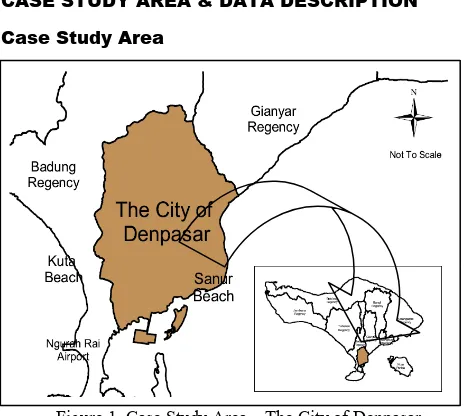
Figure 1. Case Study Area – The City of Denpasar
Province of Bali has an area of 5,634.40 km2 and a po-pulation of about 3.4 million. The island is widely known as a tourist destination. Most of popular tourist destinations are also located in southern areas including Kuta, Sanur, and Nusa Dua. Therefore, these areas are the most densely populated than any other parts of Bali. The capital city Denpasar is also located in the southern Bali as shown in Figure 1. The city of Denpasar has an area of 127 km2 with the population of 608,595[5].
Data Description
The proportion of motorcycle in the city Denpasar account-ed for about 81% of total registeraccount-ed vehicles and motorcycle accidents were reported about 67% of motor vehicle accidents [4]. Figure 2 shows motorcycle accident during period 2006-2008 in the city of Denpasar. It shows that the number of motorcycle accidents increased about 61% from 2006 to 2007 and decreased slightly about 7% from 2007 to 2008. This declining motorcycle accidents perhaps because of the safety riding campaign in Bali which was commenced in 2007. The proportion of motorcycle fatal accidents for 2006, 2007 and 2008 were 38%, 29% and 32% respectively. Thus, the average motorcycle fatal accident were 33% during period 2006-2008.
Figure 2. Road Accidents Based on Modes of Transport
MODEL DEVELOPMENT
Predictors in this study represented the characteristics of local household in the city of Denpasar including motorcycle ownership, the structure of household (ages, number of children, number of dependents, employment), total household income per month, total travel distance by all household’s members and fuel cost for number of motorcycle(s) owned by the household. Choices for motorcyclist to reduce the probability involving in slight injuries due to motor vehicle accidents were represented with two WTP scenarios. These scenarios comprise motorcyclists paying the amount of Rp. 900,000 p.a and Rp. 650,000 p.a for 25% and 15% slight injuries reductions respectively. The former WTP is based on the assumption that a motorcyclist’s WTP such amount of money (price in 2008) for motorcycle maintenance costs using genuine spare parts, while the latter is for the imita-tion ones. These maintenance costs include replacement on en-gine oil, a spark-plug, brake disks, clutch, tires, turn indicators, and a battery.
In this study, accident factors including human, vehicles, roads and environment were considered evenly to influence acci-dents occurrences. For instance, a vehicle was a factor contri-buted 25% to accidents occurrence. Consequently, a regular maintenance using a genuine spare parts would result a proper motorcycle condition. This is assumed relevant for 25% motor-cyclist’s slight injury reduction. Meanwhile, based on interviews conducted on some mechanics, the imitation spare parts conside-red to worth as half as the genuine ones. Once motorcyclists pre-fer to use the imitation spare parts, that would be considered rele-vant for 15% motorcyclist’s slight injury reduction.
Figure 3. Motorcyclists’s Willingness To Pay
For model development, response variables were scenarios 1 and 2 representing motorcyclist’s WTP for 25% and 15% slight injury reductions respectively as shown in Figure 3. These scenarioes were binominal in nature. The figure shows that 66% respondent have chosen scenario 1 (yes) or scenario 2 (no) and 34% for scenario 1 (no) or scenario 2 (yes). In other words, 66% of the respondent are willing to pay such amount of money for 25% slight injury reduction. The independent variables were continuous (age, number of workers and travel distances) and categorical for the rest. In order to represent categorical variables, dummy variables are created following the coding system in SPSS, software used in this study. Study variables and their co-ding are shown in Table 1.
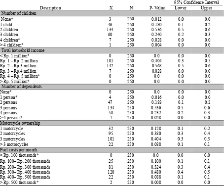
According to data related statistics shown in Table 3, some variable categories (classifications) can be neglected because of their small proportion. The hypothesis testing technique for pro-portions was used in this study to decide whether a classification could be reduced. The following typical test was used: H0: pi = 0
and Ha: pi
≠
0, where, pi is the proportion of a variableclassi-fication.
For continous independent variables, multicollinearity test were undertaken to ensure that these variables significantly inde-pendent to each other. As shown in Table 2, none of values higher than 0.8, hence multicollinearity was not a problem.
0 50 100 150 200 250 300
2006 2007 2008 Year
N
u
m
b
er
o
f acc
id
en
ts
MC Fatal Non Fatal
66% 34%
Scenario 1 (Yes) Scenario 1 (No)
34%
66%
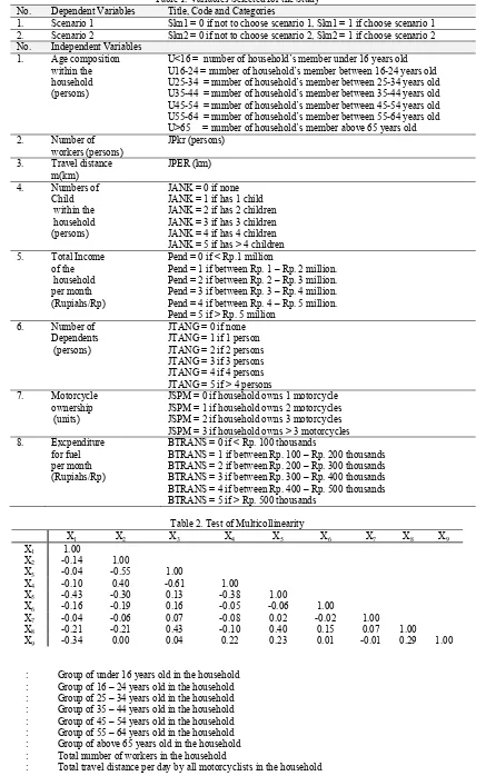
Table 1. Variables Selected for the Study No. Dependent Variables Title, Code and Categories
1. Scenario 1 Skn1 = 0 if not to choose scenario 1, Skn1 = 1 if choose scenario 1 2. Scenario 2 Skn2 = 0 if not to choose scenario 2, Skn2 = 1 if choose scenario 2 No. Independent Variables
1. Age composition within the
household (persons)
U<16 = number of household’s member under 16 years old U16-24 = number of household’s member between 16-24 years old U25-34 = number of household’s member between 25-34 years old U35-44 = number of household’s member between 35-44 years old U45-54 = number of household’s member between 45-54 years old U55-64 = number of household’s member between 55-64 years old U>65 = number of household’s member above 65 years old
2. Number of
workers (persons)
JPkr (persons)
3. Travel distance m(km)
JPER (km)
4. Numbers of
Child within the household (persons)
JANK = 0 if none JANK = 1 if has 1 child JANK = 2 if has 2 children JANK = 3 if has 3 children JANK = 4 if has 4 children JANK = 5 if has > 4 children 5. Total Income
of the household per month (Rupiahs/Rp)
Pend = 0 if < Rp.1 million
Pend = 1 if between Rp. 1 – Rp. 2 million. Pend = 2 if between Rp. 2 – Rp. 3 million. Pend = 3 if between Rp. 3 – Rp. 4 million. Pend = 4 if between Rp. 4 – Rp. 5 million. Pend = 5 if > Rp. 5 million
6. Number of
Dependents (persons)
JTANG = 0 if none JTANG = 1 if 1 person JTANG = 2 if 2 persons JTANG = 3 if 3 persons JTANG = 4 if 4 persons JTANG = 5 if > 4 persons 7. Motorcycle
ownership (units)
JSPM = 0 if household owns 1 motorcycle JSPM = 1 if household owns 2 motorcycles JSPM = 2 if household owns 3 motorcycles JSPM = 3 if household owns > 3 motorcycles 8. Excpenditure
for fuel per month (Rupiahs/Rp)
BTRANS = 0 if < Rp. 100 thousands
BTRANS = 1 if between Rp. 100 – Rp. 200 thousands BTRANS = 2 if between Rp. 200 – Rp. 300 thousands BTRANS = 3 if between Rp. 300 – Rp. 400 thousands BTRANS = 4 if between Rp. 400 – Rp. 500 thousands BTRANS = 5 if > Rp. 500 thousands
Table 2. Test of Multicollinearity
X1 X2 X3 X4 X5 X6 X7 X8 X9
X1 1.00
X2 -0.14 1.00
X3 -0.04 -0.55 1.00
X4 -0.10 0.40 -0.61 1.00
X5 -0.43 -0.30 0.13 -0.38 1.00
X6 -0.16 -0.19 0.16 -0.05 -0.06 1.00
X7 -0.04 -0.06 0.07 -0.08 0.02 -0.02 1.00
X8 -0.21 -0.21 0.43 -0.10 0.40 0.15 0.07 1.00
X9 -0.34 0.00 0.04 0.22 0.23 0.01 -0.01 0.29 1.00
Where
X1 : Group of under 16 years old in the household
X2 : Group of 16 – 24 years old in the household
X3 : Group of 25 – 34 years old in the household
X4 : Group of 35 – 44 years old in the household
X5 : Group of 45 – 54 years old in the household
X6 : Group of 55 – 64 years old in the household
X7 : Group of above 65 years old in the household
X8 : Total number of workers in the household
Table 3. Hypothesis Testing: Data Statistics
Description X N P- Value
95% Confidence Interval Lower Upper
Number of children
None* 3 250 0.012 0.0 0.0
1 child 46 250 0.180 0.1 0.2
2 children 134 250 0.536 0.5 0.6
3 children 60 250 0.240 0.2 0.3
4 children* 7 250 0.028 0.0 0.0
> 4 children* 1 250 0.004 0.0 0.0
Total household income
< Rp. 1 million* 0 250 0.0 0.0 0.0
Rp. 1 – Rp. 2 million 101 250 0.404 0.3 0.5
Rp. 2 – Rp.3 million 142 250 0.568 0.5 0.6
Rp. 3 – Rp.4 million 7 250 0.028 0.0 0.0
Rp. 4 – Rp. 5 million* 0 250 0.0 0.0 0.0
> Rp. 5 million* 0 250 0.0 0.0 0.0
Number of dependents
None* 0 250 0.0 0.0 0.0
1 person* 4 250 0.016 0.0 0.0
2 persons 47 250 0.188 0.1 0.2
3 persons 134 250 0.536 0.5 0.6
4 persons 58 250 0.232 0.2 0.3
> 4 persons* 7 250 0.028 0.0 0.0
Motorcycle ownership
1 motorcycle 32 250 0.128 0.1 0.2
2 motorcycles 95 250 0.380 0.3 0.4
3 motorcycles 101 250 0.404 0.3 0.5
> 3 motorcycles 22 250 0.088 0.1 0.1
Fuel costs per month
< Rp. 100 thousands* 0 250 0.0 0.0 0.0
Rp. 100– Rp. 200 thousands 25 250 0.100 0.1 0.1
Rp. 200– Rp. 300 thousands 81 250 0.324 0.3 0.4
Rp. 300– Rp. 400 thousands 120 250 0.480 0.4 0.5
Rp. 400– Rp. 500 thousands 22 250 0.088 0.1 0.1
> Rp. 500 thousands* 2 250 0.008 0.0 0.0
* Statistically insignificant at the 5% level; the 95% confidence limits include 0. where: X = number of classification (yes=1), N = sample size
Based on the test, there were two categories of number of children excluded from the model development stage including ‘4 and more than 4 children’. This exclusion is carried out with merging and putting these categories as reference for the rest of classification within each variable. For instance, within number of children factor, ‘4 and more than 4 children’ were merged with ‘3 children’ and generated a new category ‘
≥
3 children’. In addition to total household income factor, ‘< Rp. 1 million’ was merged with ‘Rp. 1-2 million and generated ‘< Rp. 2 million’. Categories ‘Rp.4-5 million and ‘> Rp. 5 million’ were merged with ‘Rp.3-4 million’ and generated a new category ‘≥
Rp.3 million’.. For number of dependent factor, categories ‘none’ and ‘1 person’ were merged with ‘2 persons’ and generated a new category ‘< 2 persons’. Category ‘> 4 persons’ was merged with ‘4 person’ and generated a new category ‘≥
4 persons’. For fuel costs factor, category ‘< Rp. 100 thousands’ was merged with ‘Rp.100-200 thousands’ and generated a new category ‘ < Rp. 200 thousands’. Category ‘> Rp.500 thousands’ was merged with ‘Rp.400-500 thousands’ and generated a new category ‘≥
Rp. 400 thousands’.The entry method of logistic regression was followed using SPSS version 15. The Omnibus Tests of motorcycle fatal
accidents model coefficients is analysed in order to assess whe-ther data fit the model as shown in Table 4. The specified model is significant (Sig. < 0.05) so it is concluded that the independent variables improve on the predictive power of the null model.
Table 4. Omnibus Tests of Model Coefficients
Motorcycle fatal accidents
Chi-square Sig.
Model 31.326 .000
Table 5 contains the two pseudo R2 measures that are Cox and Snell and Nagelkerke. The former measure frequently does have a maximum less than one. It is therefore usually better to assess Nagelkerke’s measure as this divides Cox and Snell by the maximum to give a measure that really does range between zero and one. In this example, both scenarios explain 16% of the variance in the dependent variable. In addition, Hosmer-Lemeshow (H-L) test shows the significance of the developed logistic regression models (Sig. > 0.05).
Pseudo R2 Test
-2 Log likelihood Cox & Snell R2 Nagelkerke R2
Scenarios 1 and 2 289.192 0.118 0.163
Hosmer and Lemeshow Test (H-L Test)
Chi-square df Sig. (p-value)
Scenarios 1 and 2 10.011 8 .264
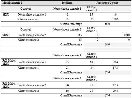
Table 6 gives the overall percent of cases that are correctly predicted by the full model. The percentages have increased from 66.0 to 67.6 for both models.
Table 6. Classification Accuracy
Model Scenario 1 Predicted Percentage Correct
Observed Not to choose scenario 1 Choose scenario 1
SKN1 Not to choose scenario 1 0 85 .0
Choose scenario 1 0 165 100.0
Overall Percentage 66.0
Observed Not to choose scenario 2 Choose scenario 2
SKN2 Not to choose scenario 2 165 0 100.0
Choose scenario 2 85 0 .0
Overall Percentage 66.0
Not to choose scenario 1 Choose scenario 1 Full Model
SKN1 Not to choose scenario 1 25 60 29.4
Choose scenario 1 21 144 87.3
Overall Percentage 67.6
Not to choose scenario 2 Choose scenario 2 Full Model
SKN2 Not to choose scenario 2 144 21 87.3
Choose scenario 2 60 25 29.4
Overall Percentage 67.6
RESULTS AND DISCUSSIONS
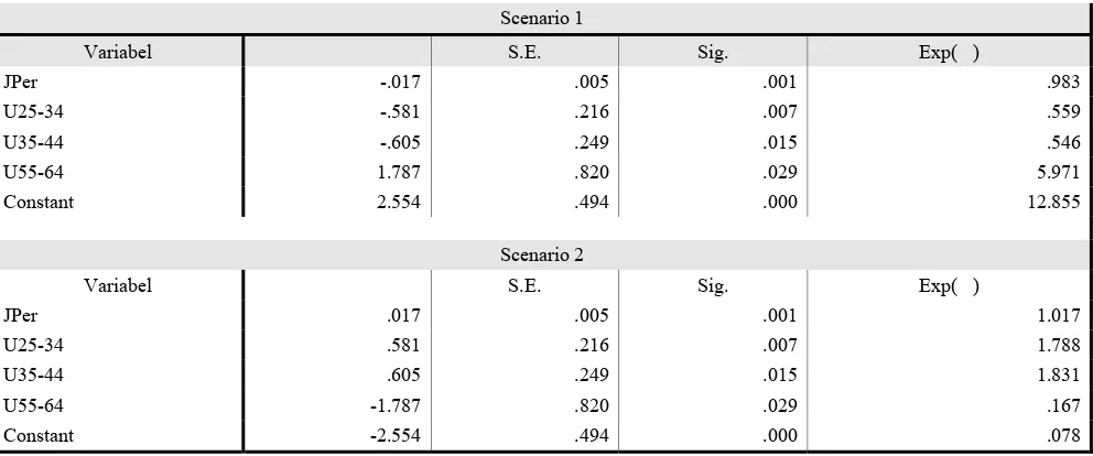
Table 7 indicate that multicollinearity was not detected since all standard errors (S.E) value were less than 2.0 for both scenarios [6]. The model results shows that at 95% confidence level, total travel distance per day by all motorcyclists in the household, motorcyclists aged between 25 and 34 years old and between 35 and 44 years old in the household were negatively related to motorcyclist’s WTP for 25% reduction in slight injuries while group of motorcyclists aged between 55 and 64 years in the household were positively related to WTP for 25% reduction in slight injuries. These were opposite to motorcyclist’s WTP for 15% reduction in slight injuries.
The scenario 1 results indicated that total travel distance per day by all motorcyclists in the household influenced about 50% on motorcyclist’s WTP for 25% reduction in slight injuries.
The equation used to arrive such values is
=
−
p
p
1
exp. (JPer)
=0,983, which resulting p = 0.496. In addition, groups of motorcyclists aged between 25 and 34 years old, between 35 and 44 and between 55 and 64 years old in the household influenced
about 36%, 35% and 86% respectively on WTP for 25% reduction in slight injuries.
The scenario 2 results indicated that total travel distance per day by all motorcyclists in the household, groups of motor-cyclists aged between 25 and 34 years old, between 35 and 44 and between 55 and 64 years old in the household influenced about 50%, 64%, 65% and 14% respectively on WTP for 15% reduction in slight injuries.
Meanwhile, total travel distance per day by all motor-cyclists in the household shared equal probabilities in influencing motoryclist’s WTP for both 15% and 25% slight injury reduc-tions. In addition, groups of motorcyclist aged between 55 and 64 years old prefered 25% to 15% slight injury reduction compared with younger motorcyclists i.e between 25 and 34 years old and between 35 and 44 years old. The high value of constant (
±
2.55) indicated that there were some other significant factors that may influence motorcyclist’s WTP for slight injuries re-duction.reduction. This is consistent with previous study conducted in the city of Surabaya, East Java, Indonesia [8] which found that ages were significant factor of WTP for motorcycle slight accident re-duction. Furthermore, introducing an educational campaign or an awareness programs about the risk of motorcycle accident is necessary, in particular for younger persons. In order to carry out
such programs, coordination among educational institution, the police and department for transport would be an advantage to prevent motorcycle accidents.
Table 7. Estimation Results Scenario 1
Variabel S.E. Sig. Exp( )
JPer -.017 .005 .001 .983
U25-34 -.581 .216 .007 .559
U35-44 -.605 .249 .015 .546
U55-64 1.787 .820 .029 5.971
Constant 2.554 .494 .000 12.855
Scenario 2
Variabel S.E. Sig. Exp( )
JPer .017 .005 .001 1.017
U25-34 .581 .216 .007 1.788
U35-44 .605 .249 .015 1.831
U55-64 -1.787 .820 .029 .167
Constant -2.554 .494 .000 .078
Where:
S.E = standard error
Sig = p- value = significance level
Jper = Total travel distance per day by all motorcyclists in the household U25-34 = Group of 25 – 34 years old in the household
U35-44 = Group of 35 – 44 years old in the household U55-64 = Group of 55 – 64 years old in the household
CONCLUSIONS
This study employes a logistic regression model to ana-lyse motorcyclist’s WTP for slight injury reduction due to motor vehicle accidents in the city of Denpasar, Bali Province. Based on the RP/SP surveys data, eight predictor variables were em-ployed in the logistic regression models. The model results found that four significant factors influenced on motorcyclist’s WTP for both 25% and 15% slight injury reduction. The analyses show that total travel distance per day by all motorcyclists in the household, groups of ages between 25 and 34 years old, between 35 and 44 and between 55 and 64 years old in the household influenced about 50%, 36%, 35% and 86% respectively on motorcyclist’s WTP for 25% slight injuries reduction and about 50%, 64%, 65% and 14% respectively on motorcyclist’s WTP for 15% slight injuries reduction.
Total travel distance per day by all motorcyclists in the househol shared equal probabilities in influencing motoryclist’s WTP for both 25% and 15% slight injury reductions. In addition, groups of motorcyclist aged between 55 and 64 years old pre-fered 25% to 15% slight injury reduction compared with younger motorcyclists i.e between 25 and 34 years old and between 35 and 44 years old. The study also found that there were some other significant factors that may influence motorcyclist’s WTP for slight injuries reduction other than these four significant factors. The result would be expected to develop strategies to prevent and reduce motorcycle accidents in Bali.
REFERENCES
O’Reilly, D., Hopkin, J., Loomes, G., Jones-Lee, M., Philips, P., McMahon, K., Ives, D., Soby, B., Ball, D., and Kemp, R. (1994). “The Value of Road Safety UK Research on the Valuation of Preventing Non-Fatal Injuries”. Journal of Transport Economics and Policy, pp. 45 – 59.
Quddus, M.A., Noland, R.B., and Chin, H.C. (2002). “An Analysis of Motorcycle Injury and Vehicle Damage Severity Using Ordered Probit Models.” Journal of Safety Research, Vol. 33, p,445-462.
Rizzi, L.I., and Ortuzar, J.D. (2006). “Road Safety Valuation Under A Stated Choice Framework.” Journal of Transport Economics and Policy, Volume 40, Part 1, pp. 69–94. State Police of Bali Province. (2008). “Accident Data Report”.
Statistics of Bali Province., 2008. Bali in Figures.
Washington, S.P., Karlaftis, M.G., and Mannering, F.l. (2003). Statistical and Econometric Methods for Transportation Data Analysis, Chapman & Hall, USA.
Widyastuti, H. and Mulley, C. (2005). “Evaluation of Casualty Cost of Motorcyclist’s SlightInjury in Indonesia.” Journal of the Eastern Asia Society for Transportation Studies, Vol.6 Widyastuti, H., Mulley, C., and Dissanayake, D. (2007). “Binary