36
CHAPTER III
RESEARCH METHODOLOGY
3.1 Population and Samples
Population is all of element that shows the special characteristic that can
use for creating the conclusion (Sanusi, 2013). The research population is all of
firm that listed in the Indonesia Stock Exchange (IDX). Base on the data of
companies that have been listed until year 2016, there are 525companies.
Based on research of AndiSupangat (2007) in AniRachmawati (2013),
Sample is the part of population that using as a research objects that taking from
the population as the representative of the population. From the population, it will
be sampled. The sample method that used in this research is using purposive
sampling. Purposive sampling is the sampling method that used some criteria to
select the samples (Amalia and Kristjiadi, 2003). The criteria that used in this
research are:
a) Manufacturing company has been listed in the Indonesia Stock Exchange
in period 2010-2015.
b) The company has been published their financial statement in period
2010-2015.
c) The company has completed data of financial statement in the Indonesia
37 3.1.1 Company as Sample
a) The manufacturing that listed on Indonesian Stock Exchange are 534
companies.
b) The manufacturing company that listed on the Indonesia Stock
Exchange (IDX) from year 2010-2015 are 51 companies.
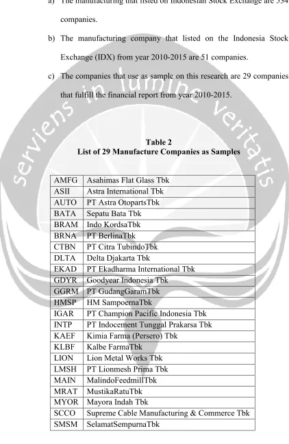
c) The companies that use as sample on this research are 29 companies
[image:2.595.89.511.119.768.2]that fulfill the financial report from year 2010-2015.
Table 2
List of 29 Manufacture Companies as Samples
AMFG Asahimas Flat Glass Tbk
ASII Astra International Tbk
AUTO PT Astra OtopartsTbk
BATA Sepatu Bata Tbk
BRAM Indo KordsaTbk
BRNA PT BerlinaTbk
CTBN PT Citra TubindoTbk
DLTA Delta Djakarta Tbk
EKAD PT Ekadharma International Tbk
GDYR Goodyear Indonesia Tbk
GGRM PT GudangGaramTbk
HMSP HM SampoernaTbk
IGAR PT Champion Pacific Indonesia Tbk
INTP PT Indocement Tunggal Prakarsa Tbk
KAEF Kimia Farma (Persero) Tbk
KLBF Kalbe FarmaTbk
LION Lion Metal Works Tbk
LMSH PT Lionmesh Prima Tbk
MAIN MalindoFeedmillTbk MRAT MustikaRatuTbk
MYOR Mayora Indah Tbk
SCCO Supreme Cable Manufacturing & Commerce Tbk
38
SQBB PT Taisho Pharmaceutical indonesiaTbk
TKIM PabrikKertas Tjiwi Kimia Tbk
TOTO PT Surya Toto Indonesia Tbk
UNIC PT Unggul Indah CahayaTbk
UNTR PT United Tractors Tbk
UNVR Unilever Indonesia Tbk
Source : www.idx.com
3.2 Data and Data Gathering
3.2.1 Type of Data
This research is using secondary data as main data which means the data
have been processed and published by partly entailed (Supranto, 1987). Secondary
data that used in this research are getting from the data that have been processed
and published by Jakarta Stock Index (IDX)
3.2.2 The Data Use in the Research
Every research exactly has variable as the item that will be run in the
research. In this research the variable that will run are the independent variable
and the dependent variable. As usually, the relation of these two variables is the
dependent variable is influence by the independent variable. The independent
variable is the capital structure. There are five the proxy of capital structure in this
research, which is Debt to Equity Ratio (DER), Debt to Equity Ratio, Debt to
Assets Ratio (DAR), Tangibility, Interest Coverage Ratio (ICR), and Financial
Leverage Multiplier (FLM). The dependent variable that use in this research is the
firm value, whereas the proxy of firm value is Price to Book Value. The data that
39
Equity Ratio, Total Liabilities and Total Assets that use to find Debt to Assets
Ratio, Total Fixed Assets and Total Assets that use to find the Tangibility,
Earning Before Interest & Tax and Interest Expense to find the Interest Coverage
Ratio, and the last are Total Assets and Share Capital that use to find The
Financial Leverage Multiplier.
3.2.3 Source of Data
The data that will run is secondary data that can be finding from the
website of the Indonesia Stock Index (IDX). The website address is
www.idx.co.id. The IDX’s website will provide the data for every each year.
3.3 Research Variable
The research variables can be separate into two parts which is independent
variable and dependent variable. Independent variable is variable that influence
the related variable. And the dependent variable is the variable that influenced by
the independent variable.
3.3.1 Independent Variable
The independent variables are variable that varied or manipulated
by the researcher. And independent variable is the presumed cause,
whereas the dependent variable is the presumed effect (Dependent and
Independent variable). And the independent variable of this study is the
capital structure. The proxy of capital structure is Debt to Equity Ratio
(DER), Debt to Assets Ratio (DAR), Tangibility, Interest Coverage Ratio
40
is finding from Total Debt divided by Equity of share holder. The Debt to
Asset Ratio is finding from Total Debt divided by Total Assets. The
Tangibility is finding from Total Fixed Asset divided by Total Assets. The
Interest Coverage Ratio (ICR) is finding from Earning before Interest and
Taxes (EBIT) divided by Interest Expenses. The Financial Leverage
Multiplier (FLM) is finding from Total Assets divided by share capital.
The formula of the independent variables:
- Debt to Equity Ratio =
Source : http://www.accountingtools.com/
- Debt to Asset Ratio =
Source :JahirulHoque, Ashraf Hosshain, Kabir Hossain, (2015)
- Tangibility =
Source :JahirulHoque, Ashraf Hossain, Kabir Hossain, (2015)
- Interest Coverage Ratio =
Source :JahirulHoque, Ashraf Hossain, Kabir Hossain, (2015)
- The Financial
LeverageMultiplier =
41 3.3.2 Dependent Variable
The dependent variable is the respond that is measured. The
dependent variable in this study is the firm value whereas the firm value
proxy is Price to Book Value. The price to book value can be getting from
the comparison of Market price per share and Book value per share.
The formula of the dependent variable:
- Price to Book value =
Source :http://www.financeformulas.net/
3.4 Method of Analysis and Hypothesis Testing 3.4.1 Multiple Linear Regressions
Analysis technique that used in this study is multiple linear regressions.
Model of equation can be written as follows (Fisher, 1922)
PBV = H+J1DER + J2DAR + J3TAN + J4ICR + J5FLM
Where:
PBV : Price to Book Value
DER : Debt to Equity Ratio
DAR : Debt to Assets Ratio
TAN : Tangibility
ICR : Interest Coverage Ratio
42
e : error
Multiple linear regressions is important as the basis for the analysis,
considering fundamental research. This method of analysis is technique to find the
relation among the variable. This means that if the coefficient b is positive (+), it
will give a one direction impact between the independent variable with the
dependent variable, any increase in the value of independent variable will lead to
increase the dependent variable. Vice versa, if the coefficient value of n is
negative (-), it indicates a negative effect which increase the value of the
independent variable will result in impairment of the decrease in the dependent
variable.
3.4.2 Classical Assumption Test
The test will test the statistic of the data based on the multiple linear
regression using Ordinary Least Square (OLS) that generate Best Linear Unbias
Estimator (BLUE). To identify and emphasize the relation of the data, the data of
the research must be following the Classical Assumption Test. whereas: (Novi
RehulinaSitepu, 2015)
1. Normality Test
This will test the residual value of that generate from the regression
have a normal distribution or not. This test common use in the parametric
statistic analysis good regression model will have residual value that
distributed normally. To do the normality test the analysis is histogram,
probability plot, and also Kolmogorov-Smirnov Z test. With knowing the
43
the average and median. We could know the normality from histogram
Figure by seeing the form of the Figure if it forms a mountain then the
distribution is normal. In the P-P Plot Figure, if the dot spreading near the
diagonal the data is normal. Using Kolmogorov-Smirnov Z the
significance should higher than 0.05.
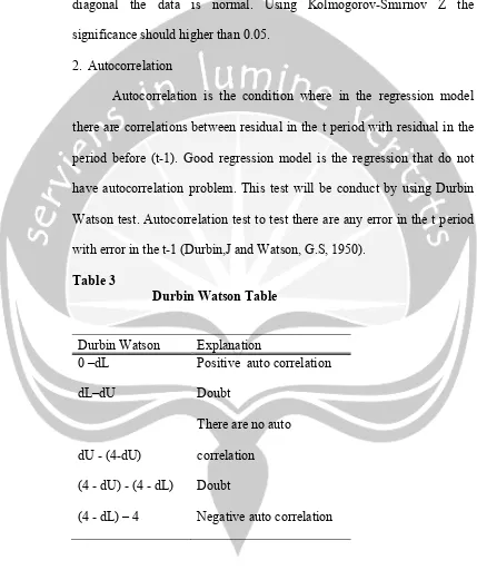
2. Autocorrelation
Autocorrelation is the condition where in the regression model
there are correlations between residual in the t period with residual in the
period before (t-1). Good regression model is the regression that do not
have autocorrelation problem. This test will be conduct by using Durbin
Watson test. Autocorrelation test to test there are any error in the t period
[image:8.595.84.513.171.692.2]with error in the t-1 (Durbin,J and Watson, G.S, 1950).
Table 3
Durbin Watson Table
Durbin Watson Explanation
0 –dL Positive auto correlation
dL–dU Doubt
dU - (4-dU)
There are no auto
correlation
(4 - dU) - (4 - dL) Doubt
(4 - dL) – 4 Negative auto correlation
44
Multicollinearity is the condition where in the regression model
there are perfect correlations or perfect approach among the independent
variable. In the good regression model it should be no perfect correlation.
Statistic tool that often use to test the disruption of multicollienearity are
Varian inflation factor (VIF), person correlation among independent
variable, or seeing the eigenvalues and condition index (CI). Test
Multicollinearity using tolerance and variant inflation factor (VIF) in the
regression model or by compare the individual coefficient determinant (r2)
with the determinant value all at one (R2). To test the multicollinearity we
could see from the tolerance and VIF. Tolerance will measure the
variability of independent variable that not be explained by the other
independent variable. So the low tolerance levels same with the high VIF.
Cutoff value that commonly use to show there are multicollinearity is
tolerance <0.10 or same with VIF>10. (Ghozali, 2006).
4. Heteroscedasticity Test
Heteroscedascity test aims to test whether the model regression
occur inequality residual variance of one observation to other observation.
A good regression model is going homocedasticity or that are no
hetercedasticity. Detect the heterocedasticity done by seeing Figure plots
from the value prediction of the dependent variable with the residual. With
basic analysis:
1. If there are certain patterns, such as dots that form a pattern particular,
regular (corrugated, wide, and narrowing), it has been indicated
45
2. If there is no particular pattern and the points spread above and below
zero on the Y axis, there will be no heterocedasticity.
Analysis of the Figure plot has significant drawbacks because the
number of observation affects the result plot. More and more small
number of observations, the more difficult to interpreted the Figure plot.
3.5 Hypothesis Testing
Hypothesis testing is the use of statistics to determine the probability that a
given hypothesis is true.
1). Thehyphothesis formula will be used to examine the hyphothesis of this
research are;
H0: The Capital Structure does not impact the Firm Value
H1: The Debt to Equity Ratio has positive impact on Firm Value
H2: The Debt to Assets Ratio has negative impact on Firm Value
H3: The Tangibility has positive impact on Firm Value
H4: The Interest Coverage Ratio has positive on Firm Value
H5: The Financial Leverage Multiplier has positive impact on Firm Value
The examination will use the multiple Regression Analysis result. The condition
of examination will be used to approve or reject the H1, H2, H3, H4, H5.
If p<Hthe H1,2,3,4,5 will be approve and H0will be rejected; but if p>Hthen
46
Where the alpha is 0.05 that the observed effect is statistically significant, the null
hypothesis is ruled out, and the alternative hypothesis is valid.
2). t-Value Testing
T-Value Testing is using to test the influence of independent variable to
the dependent variable partially. This testing method use to compare the t-count to
the t-table.
3). F-Value Testing
F-Value Testing is using to test the influence of independent variable to
the dependent variable simultaneously. This testing method use to compare the
F-count to the F-table.
4). Adjusted R2
Coefficient Determination (R2) used to measure the ability of the model in
explaining the variation in the dependent variable. The coefficient of
determination can be searched by the formula (Gujarati, 1999):
Coefficient determination is between 0 and 1. R2values are small, means
that ability of the independent variable in explaining the dependent variable is
very limited (Ghozali, 2005). Value close to 1 means that the independent variable
gives almost all the information needed to predict the variation of the variable