Electric Power Systems Research81 (2011) 1363–1372
Contents lists available atScienceDirect
Electric Power Systems Research
j o u r n a l h o m e p a g e :w w w . e l s e v i e r . c o m / l o c a t e / e p s r
Statistical appraisal of economic design strategies of LV distribution networks
Chin Kim Gan
∗, Pierluigi Mancarella, Danny Pudjianto, Goran Strbac
Department of Electrical and Electronic Engineering, Imperial College London, South Kensington Campus, SW7 2AZ London, UK
a r t i c l e
i n f o
Article history:
Received 10 September 2010
Received in revised form 12 January 2011 Accepted 1 February 2011
Available online 1 March 2011
Keywords:
Network design policy Distribution losses Distribution system analysis Life cycle cost (LCC)
a b s t r a c t
This paper presents a statistical approach for assessing general LV distribution network design strategies based on a large set of realistic test networks and optimal economic circuit design. The test networks are generated using a fractal-based algorithm that allows creation of generic networks with various topological features (e.g., typical of rural/urban/mixed areas) and characterised by different numbers of substations, numbers of customers, load densities, and so forth. In comparison to standards derived from a traditional approach, that is, case studies on a small number of specific real or test networks, the proposed approach facilitates the derivation of more robust conclusions on optimal network design policies and can thus be used as a valuable tool for decision support. The methodology is exemplified through numerical applications for both urban and rural areas.
© 2011 Elsevier B.V. All rights reserved.
1. Introduction
One of the main challenges for distribution network planners and operators is to develop optimal network design strategies, which involves evaluation of a wide range of options such as cable types, cable sizes, locations of substations, and types and sizes of transformers. Without general guidance as to how these choices should be made, network planners can only rely on their experi-ence. This may lead to suboptimal decisions and to inconsistent strategies that eventually will increase the network cost. However, development of general network design guides is a complex task, especially for LV systems, which have millions of different sam-ples. In addition, due to the sheer volume of network data, relevant information for LV systems is often unavailable or inadequate, and is generally insufficient for large scale network design. Thus, several works have addressed network design of specific networks[1,2]or idealised networks[3–5], incorporating existing design policies or standards and with specified load point positions and available sub-station sites. More recently, a distribution network model has been developed for large-scale distribution planning, which divides the network zone into mini-zones that are optimised independently
[6,7]. In addition to that, a reference network model which uses real
Abbreviations:ADMD, after diversity maximum demand; DSO, distribution sys-tem operator; LCC, life cycle cost; OHL, overhead line; PDF, probability density function; PMT, pole mounted transformer; UGC, underground cable.
∗Corresponding author. Tel.: +44 2075946295; fax: +44 2075946282. E-mail addresses:[email protected],[email protected](C.K. Gan), [email protected](P. Mancarella),[email protected] (D. Pudjianto),[email protected](G. Strbac).
location coordinates of final customer to automatically generate the corresponding street map for simultaneous planning of high-, medium- and low voltage networks is reported in[8]. Regarding circuit design, life cycle cost (LCC) analysis for circuits[1,3,9]and transformers [10–12]is a consolidated methodology adopted in several countries for network design. However, the adoption of LCC analysis for strategic design and assessment of different types of networks has not been previously explored.
This paper introduces a statistical approach intended to support the decision making process of network planners and operators in the identification of the best design strategy for given LV net-work types. The approach is based on synthetic input information, but could potentially be applied to a large variety of networks, thus moving beyond the current state of the art. In particular, the paper suggests an approach for strategic assessment of LV distri-bution networks using the LCC methodology of optimal network design. The LCC model illustrated here intrinsically highlights the prominent role of losses in circuit design, thus resulting into pro-motion of socially efficient investment policies and taking into account environmental concerns. The main outcomes from the analysis serve to indicate optimal network design strategies for given areas (for instance, rural or urban, depending on the specific topological features) with different load densities and charac-teristics, and identify the optimal number of substations, circuit cost breakdown (investment, maintenance and losses), and so forth.
The methodology developed here is based on the generation and analysis of a large number of statistically similar networks, with some common topological parameters. This enables deci-sion makers to draw much more robust concludeci-sions than those reached through the study of specific case study networks. A key
0378-7796/$ – see front matter© 2011 Elsevier B.V. All rights reserved.
previously in the literature.
Numerical studies are presented to illustrate the applications of the proposed methodology to both urban and rural areas, high-lighting the main features of each case and the differences between the two. In particular, the optimal number of 11/0.4 kV substations to supply areas with different load densities and a breakdown of the average costs of these networks are presented and discussed in a typical UK context.
The paper is structured as follows. Section 2 illustrates the characteristics of the tool for statistical network generation and substation placement. Section3describes the minimum LCC-based methodology used to design optimal economic circuits. Section
4presents numerical applications of the developed methodology within typical urban and rural configurations. Finally, Section5
contains concluding remarks and suggests potential future work.
2. A fractal model for statistical network creation
2.1. Fractal network generation
Consumers’ locations and network branch connections play critical roles in network design, as these affect the length of the network as well as, together with the specific demand load pat-terns, the circuit sizing. Subsequently, simple geometric models
[4]or network trees specifically generated for the lowest overall cost[5]may in general not be adequate to reproduce realistic net-work features and consumer distribution. It has also been shown that fractal models are more suitable to represent low load den-sities as compared to geometric models owing to their ability to generate realistic spatial consumer settlement with non-uniform load and supply points[15], resulting in spatial distributions of fractional dimension[16]. Building on these findings, the fractal network generation algorithm used in[17–19]is adopted in this paper to generate large sets of weakly meshed networks. However, as with the typical operation of the great majority of LV networks, further adjustments are carried out (see below) to transform the network into a number of radial ones.
2.2. Substation siting
The numberNsof MV/LV (11/0.4 kV, in typical UK cases)
distri-bution substations is an input to the model. In the methodology discussed here, substations are placed so as to be indicatively at the centre of load clusters, consistent with the general design pro-cedures in order to minimise the amount of equipment installed, losses and voltage drops[4]. A major advantage of the approach illustrated below is that the number of substations can be changed in a relatively straightforward manner, without the need for net-work reconfiguration, which allows for a better understanding of the cost of equipment, installation, maintenance, and network losses as a function of the number of substations for a given network configuration.
of the normally open points (NOPs) that would minimise losses and voltage drops. Consequently, the entire weakly meshed net-work is broken down intoNsradial networks (islands), with one
substation serving each island.
•The substation position is then iteratively and heuristically read-justed across the points available in the specific island taking into account the geometric characteristics of the feeders emanated from the substation. More specifically, with reference to one island and one substation, the final substation location is selected so as to minimise the standard deviationof the overall feeder lengths, defined as:
In(1),Nis the number of feeders from the substation,Bfis the
overall length of feederf,is the mean value ofBfover theN
feeders,Mfis the number of branches along thef-th feeder, and
Lfkis the length of branchkat feederf.
It is important to mention that the trade-off between feeder length and supplied power has been preliminarily considered at the relevant centre of load. In fact, it has been observed that readjustment of the final transformer location within the radial networks by considering the “balanced feeder” criterion gives satisfactory results. This is necessary to avoid small loads being located too far from the substation; which potentially leads to voltage problems. In this regards, rather than co-optimising num-ber and location of substations for a given specific network as for instance in[20], the proposed approach aims to analyse the impact of different network design strategies (and in particular number of substations) for a given area based on a large num-ber of statistically similar networks. In this light, while detailed substation optimisation can be performed for real networks, it is much more useful for network planners to have statistical informa-tion on alternative design policies. In reality, social, geographic and cost constraints would restrict the final selection of the substation location.
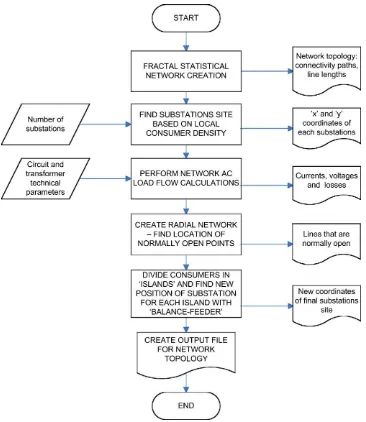
2.3. Statistical network creation algorithm
The final network topology information is saved and exported as an output file that becomes the input data to the network design module described in Section 3. The complete network creation algorithm is synthesized inFig. 2.
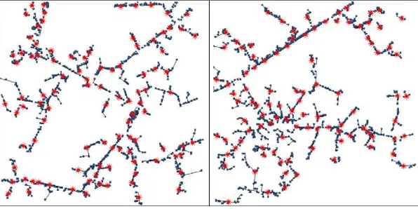
Fig. 1.Examples of a network supplied by (a) one substation and (b) six substations.
typical urban and rural networks with different seeds is shown in
Figs. 3 and 4, respectively.
The main topological difference between urban and rural net-works is driven by the consumer settlement patterns. Consumers in urban areas tend to be scattered more evenly, with relatively higher load densities. On the other hand, consumers in rural areas
tend to aggregate in a more clustered fashion (villages), with large open areas dedicated to farms, green spaces, natural reser-voirs, and so on, and consequently have relatively lower load densities.
Previous collaborations with several distribution design engi-neers had already shown that the networks generated by the fractal
Fig. 3.Statistically similar urban networks with two different seeds.
algorithm resemble real networks[18]. More recent project col-laborations with a number of DSOs in the UK have confirmed that the key statistical characteristics of the generated networks are comparable with those of real distribution networks of sim-ilar topologies, particularly in terms of the associated network lengths. More specifically, from the network data provided by DSOs, the average network length associated with a substation ground-mounted transformer (urban/semi-urban networks) in the UK system is about 1400 m, while the aggregated average network length of the distribution system modelled using the statistical net-work tool described here is about 1300 m[14]. For rural networks, the average network length associated with a PMT is about 200 m, which is again in very good match with the average real figure of about 209 m.
3. Optimal network design methodology
3.1. Load models and load flow analyses
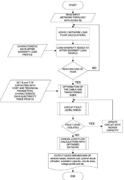
In order to design a cost-effective network, a minimum LCC methodology is adopted here. More specifically, the annuitised plant investment cost is traded off against the relevant operational costs (namely, costs due to maintenance and losses). In addition, the equipment is selected to meet specific constraints such as voltage limits[21]and security standards[22]in order to meet optimality conditions. The overall algorithm flow chart is illustrated inFig. 5, and is detailed in the sequel.
The network design and assessment carried out here begins with the analysis of time-varying demand patterns and relevant load flows, allowing more accurate results than analyses based on “aver-age” loss factors (see e.g.,[23]) or peak loads[17]only. In particular,
for economic analysis it may be crucial to address the correlation between loads (and thus losses) and the variable cost of electric-ity in the time domain. Four typical consumer types commonly found in UK networks have been considered. Given the consumer types are domestic dominated with relatively small commercial and industrial buildings, the consumer points are randomly allo-cated across the network (see Section4for details). However, for larger commercial and industrial consumers which correspond to business district or industrial estates, it will be necessary to con-sider the type of neighbourhoods while allocating these consumer points. Then, for each consumer point and for each hour, a random variation of demand around the mean value of the after-diversity profiles is applied, according to typical statistical models estimated for UK loads[24]. Hence, it is possible to model “peaky” phenomena occurring in the network for better appraisal of losses and voltage drops. For this, a classic AC load flow is performed over a one-year time span. The power factor is assumed to be constant and equal to 0.9.
3.2. Optimal circuit design: formulation of the continuous optimisation problem
For a specific circuit, once the relevant values of currentI(t) are known on an hourly basis (the time step considered in the analysis), the optimisation problem can be stated as
min Ic
(TCc)=min Ic
CCc+CMc+CLc(I(t))
(2)s.t. ˆI < Ic.
In (2), the objective function to be minimised is the circuit annual total costTCc(that is, the levelised annual cash flows[25]
corresponding to the circuit LCC over the considered life span), and
cost per circuit length.
•Total annual cost of losses CLc[
£
/year], which is a function of the average currentI(t) circulating in the circuit at the hourt(for three-phase circuits, a balanced system is assumed) according toCLc=l·Rc· 8760
t=1
I2(t)·(t) (4)
wherelis a loss-related coefficient equal to 2 for single-phase circuits and to 3 for three-phase (balanced) circuits,Rcis the
cir-cuit resistance for each phase (an average value is assumed for all phases and over the time), andis the estimated specific cost of losses [
£
/MW h] at the hourt.The constraint in(2)refers to the thermal condition whereby the peak current ˆImust be lower than the derived optimal circuit capacityIc.
One reference year is considered in this paper, with a focus on comparative assessment of different network characteristics and design strategies. Inclusion in the model of further parameters more relevant to network planning issues, such as load or energy cost increase/decrease across multiple years, will be object of future investigations.
Given a particular family of circuits (e.g., “Wavecon” cables[27]) the total cost(2)can be rewritten as a function of the circuit charac-teristics, and a closed-form expression for the continuous optimal circuit capacityIccan be derived, as illustrated in[28]. The result-ing values of circuit utilisation (defined as the ratio of circuit peak current to circuit optimal ampacity) for both underground cables (UGC) and overhead lines (OHL) for LV networks are typically quite low, in the range 15–25% for UGC and 10–15% for OHL. Hence, cir-cuit design thermal constraints are generally non-binding, in line with findings that highlight the prominent role of losses in network economic[29,30]as well as environmental design[31,32].
3.3. Optimal network design: discrete optimisation
While the model(2)is valid for the design of a specific circuit, for network assessments the LCC optimisation problem as stated above needs to be extended to the network under consideration and can be written as
min(TCN)=min
work. The sum is over the overall number of circuitsNNin the
network, and for each circuit ithe optimal capacity Iic must be selected from the setCof available capacities for the considered cir-cuit type. Typical network constraints include voltage and thermal limits and fault level requirements, as illustrated below.
in practice to good results[28].
Once the optimal continuous circuit capacity has been calcu-lated for each circuit in(6)through the model(2), the adjacent upper and lower capacity values from the setCare analysed. More specifically, for both these capacities the total cost(6)is calculated on the basis of the known branch current and the other input data, and the capacity yielding the overall minimum cost is selected as the optimal one (discrete optimisation). For larger capacity values, the capacities inCrefer to several circuits in parallel.
3.4. Optimal transformer design
An equivalent problem(6)is also solved for substation trans-formers with the objective of minimising the annual total costTCT
for all network transformers, namely,
min(TCT)=
In(7),SjTis the optimal transformer capacity [kV A] selected for each substationjfrom a set of available capacitiesT, with the con-straint that this capacity has to be higher than the power peak ˆSjT. The transformer capacities can refer to several units in parallel. The components (all expressed in [
£
/year]) of the total costTCTj in(8)are as follows for a given transformerj:
•Annuitised capital costCCj T=A·IC
j
T,withIC j
T being the trans-former investment cost.
•Annual cost of maintenanceCMj
T(again to be defined case by case given the specific problem).
•Annual cost of lossesCLj
T,in turn expressed as
CLjT=LCLjT+NLCLTj =
In(8), the termLCLTjrepresents the cost of transformer load losses over one year, withRjT being the transformer phase resistance andIjT(t) the hourly phase current. The termNLCLjT represents the annual cost of no-load losses, given by the core iron losses PjFe[W], assumed to be constant, weighted by the specific hourly cost of losses(t).
0
Fig. 6.Percentage of violated cases for the 5 MV A/km2case.
3.5. Fault level checks
After determining the optimal circuit capacities throughout the network, fault studies are carried out to determine the maximum through-fault current for every line, in line with standard proce-dures[33]. The maximum short-circuit current is calculated for each node starting from the 0.4 kV busbar of each substation (infeed node). The value of this current must be lower than the permitted short-circuit current of any of the lines connected to that node. If this is not the case, the line is replaced by one with a higher cross-section, which also exhibits a higher permitted short-circuit current. Moving downstream through the network, the check is repeated until all lines are examined and all fault current con-straints are successfully met.
3.6. Methodology for the identification of the optimal number of substations
In order to identify the optimal number of substations min-imising the overall network cost for a given load configuration, parametric analyses are run by changing the number of substations Nsacross a suitable range. For each specific number of substations
considered, the design algorithm illustrated inFig. 5is applied. The increment inNsis set to approximately 10% of the heuristically
estimated (based on experience and preliminary studies) optimal number of substations. For each of the identified candidate sets, 1000 seeds are simulated so as to build a statistical representa-tion of the results. At this stage, the maximum/minimum voltages up to the service cut-out point (consumer point) are checked to give an indication of the suitability of given configurations to oper-ate within statutory limits (+10%/−6% of the nominal voltage[21]). Given the high-level nature of the strategic studies conducted here (voltage control mechanisms are not modelled), the impact of volt-age constraints is considered from a statistical point of view. More specifically, for a given load density and number of substations, the alternative under examination is considered statistically strong enough in terms of voltage profiles based on a certainnon-exceeding probabilityof cases (corresponding to different seeds) for which the constraints are not met. A threshold of 10% has been selected, a figure that is generally accepted as reasonable for such strate-gic studies. Hence, for a given load density, in order to consider a particular number of substations as a potential candidate for the optimal network design, no more than 10% of the simulated seeds should exhibit voltage violations. For instance,Fig. 6shows a typ-ical voltage violation probability profile for a given load density (namely, 5 MV A/km2) in urban areas, as a function of the number of substations. The number of violations decreases as the num-ber of substations rises, with the decrease becoming less evident
0
Fig. 7. Distribution of minimum voltages for the case 5 MV A/km2, 24 substations, 1000 seeds.
when the substation number becomes large enough to avoid volt-age problems.
Figs. 7 and 8show the probability density function (PDF) of the minimum voltage and of the total network cost for the case of 24 substations supplying a specific load of 5 MV A/km2. Here, only about 8.5% of the seeds generate a network with violation of the minimum voltage limit, making this configuration a candidate for optimality.
Once the subset of potential numbers of substations meeting the network design constraints for given load characteristics is estab-lished, the configuration exhibiting the minimum LCC is chosen as optimal (themean valueof the network LCC is considered here as the metric to compare different alternatives).
4. Numerical applications
4.1. Description of the case studies
A number of case studies have been carried out with reference to typical UK urban and rural networks. Each case uses a settlement of 2000 consumers have been considered and an increase in the value of load density has been achieved by decreasing the size of the relevant area. Then, for each load density case, the number of substations has been modified so as to identify the relevant impact on cost and other indicators. For each configuration analysed (load density and number of substations), simulations have been run for
0
0
Load density (MVA/km²)
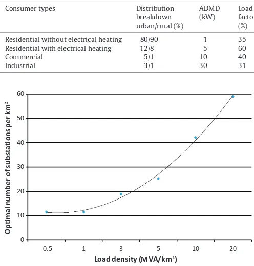
Fig. 9.Optimal number of substations density as a function of load density for urban areas.
one thousand seeds, corresponding to one thousand statistically similar networks (see for instance the two examples inFig. 2).
Four characteristic user types have been used, as mentioned in Section3.Table 1shows the user distribution breakdown and their relevantADMDand load factor. Urban networks are assumed to be supplied only by UGC and indoor substations, whereas rural networks use OHL and pole mounted transformers (PMT).
4.2. Results for urban areas
The optimal number of substations per km2 for given load density values for urban areas is presented in Fig. 9. The over-all trend can be approximated well with a second order function. It should be noted that for the lower load densities the optimal number of substations per km2saturates and does not change sig-nificantly, owing to arising voltage drop constraints. For higher load densities, voltage drops are not an issue as consumers are sited relatively close to the feeding substation, but an increas-ing number of substations per km2 is needed to economically meet the network demand. A synthetic summary of the main results for optimal configurations for the load densities consid-ered in the analysis is given in Table 2. Typical average urban load densities in the UK are in the range 3–8 MV A/km2. Here, the load densities considered span a wide set of scenarios, from
0
Load density [MVA/km²]
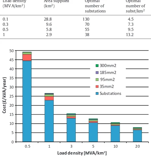
Fig. 10.Breakdown of equipment and losses average costs, including cable instal-lation costs, as a function of load density.
suburban areas (1 MV A/km2, with 0.5 being an extreme case closer to the situation in rural settlements) to city centre areas (20 MV A/km2).
Fig. 10shows the breakdown of the average cost of equipment and losses, including cable installation costs (in
£
/kV A/year), for the optimal number of substations identified for different load densities. The overall network cost is mainly determined by the extremely high UGC installation cost in UK urban areas, followed by the cost of indoor substations, while losses do not have a major influence. The difference in the cost per kV A increases with decreasing load density, mainly due to longer network lengths, which brings about higher UGC installation costs, and to voltage drop issues, which on average call for the use of more substations per area unit. From the more detailed equipment cost breakdown inFig. 11, it can be seen that substation cost dominates UGC cost and rises exponentially with a decrease in the load density, as the specific number of substations increases. The overall cost of cables is relatively low compared to the other costs, so that investment in relatively losses-driven high cross-sectional cables is even more justified.A breakdown of the average losses (as a percentage of the over-all energy demand) for different load densities in the case of the optimal number of substations is shown inFig. 12. Overall, losses are relatively low owing to use of the optimal design strategy. Transformer losses make up about 60% of the overall losses, with a substantial share due to core losses, higher for decreasing load den-sity (due to the higher number of substations). This highlights the additional potential to decrease losses by adopting high-efficiency transformers.
With an increase in load density, voltage drop constraints are less binding, and this leads to saturation in the needed number of substations. Therefore, the number of consumers supplied from a given substation increases (Table 2). However, at the same time, the average transformer size increases as well. Indeed, it should
Table 2
Optimal number of substations, total costs, average transformer sizes and losses in urban areas.
Table 3
Optimal number of substations, total costs, average transformer sizes and losses in rural areas.
Load density
Load density [MVA/km²]
300mm2
185mm2
95mm2
35mm2
Substations
Fig. 11.Breakdown of the average equipment cost for different load densities.
be highlighted that the main constraint for high load densities in urban areas is the maximum available size of transformer, typically equal to 1 MV A.
4.3. Results for rural areas
The average load density for UK rural areas is approximately 0.17 MV A/km2 [18]. However, load densities vary depending on the type and geographic characteristics of the area considered, and so rural load densities ranging from 0.1 to 1 MV A/km2have been analysed here. A similar network design procedure and analysis to the urban case have been performed for the rural case. Due to space limitations, only a few synthetic results for the optimal configura-tions found for various load densities are presented inTable 3. As in the urban case, the cost of supplying consumers decreases sub-stantially with an increase in the load density. However, for a given
0.0
Load density [MVA/km²]
Circuit Losses
Tx Iron Losses
Tx Cu Losses
Fig. 12.Breakdown of the average losses for different load densities.
load density (for instance 0.5 and 1 MV A/km2) the total network cost to supply urban areas is about six times higher than for rural areas, owing to higher costs of indoor substations and, above all, the extremely high cable excavation cost in urban areas.
The binding network design constraint in rural areas appears to be voltage-related, as opposed to urban areas for which thermal constraints are generally more binding (as feeders are relatively shorter and more heavily loaded). In fact, the results suggest that in rural areas it is necessary to increaseNs, which essentially reduces
the length of the OHL feeders associated with each transformer, so as to alleviate voltage drop issues. Hence, in order to supply a given number of consumers, rural areas would need many more transformers than urban areas.
5. Conclusions
This paper has introduced a statistical methodology for the generic appraisal of different LV distribution network design strate-gies that is suitable for decision making on large scale applications. In contrast to a traditional approach where the assessment is car-ried out based only on a small number of specific networks, the methodology developed here allows for the analysis of a large num-ber of test networks generated through a fractal-based algorithm. The circuit design methodology adopts a minimum LCC approach for selecting the optimal size of conductors and transformers, and implicitly takes into account losses as a key driving factor for net-work investment, especially at LV where the great majority of losses occur. Numerical applications for urban and rural areas have been presented in order to illustrate a number of potential applications. These include investigation of the optimal number of substations for different load densities and topologies, and identification of typ-ical cost breakdown trends for different network characteristics, so as to highlight the key drivers of improved network economic per-formance. The proposed model thus not only represents a valuable tool for decision support in the development of LV network design strategies, but could also be used to identify generic “reference net-works”, for instance for policy development purposes.
Work in progress includes extension of the model to the anal-ysis of upstream voltage levels, and assessment of the impact of distributed energy resources on optimal network design practices.
Acknowledgements
Chin Kim Gan would like to gratefully acknowledge the financial support of Universiti Teknikal Malaysia Melaka and the Ministry of Higher Education of Malaysia for his PhD study at Imperial College London.
Appendix A. Nomenclature
A.1. List of symbols
A annuity present worth factor
Ic circuit optimal current-carrying capacity [A]
IT transformer hourly phase current [A]
ICc circuit investment cost [
£
]ICT transformer investment cost [
£
]j (superscript) transformer index
k (superscript) branch index
l loss-related coefficient
L length of branch at considered feeder [km]
LCLT cost of transformer load losses [
£
/year]n network technical/economic life [years]
N number of feeders from a substation
NS number of substations
NN number of circuits in the network
NT number of transformers in the network
NLCLT annual cost of transformer no-load losses [
£
/year]PFe transformer core iron losses [W]
Rc circuit resistance []
RT transformer phase resistance []
ST optimal transformer capacity [kV A]
ˆ
ST transformer peak capacity [kV A]
T set of available capacities for a given transformer type TCc circuit annual total cost [
£
/year]TCN annual total cost of all network circuits [
£
/year]TCT transformer annual total cost [
£
/year]mean value ofBover the considered feeders
(t) cost of losses at hourt[
£
/MW h]standard deviation of the overall feeder lengths
References
[1] M. Ponnavaikko, K.S. Prakasa Rao, An approach to optimal distribution system planning through conductor gradation, IEEE Transactions on Power Apparatus System 101 (1982) 1735–1742.
[2] Z. Sumic, S.S. Venkata, T. Pistorese, Automated underground residential distri-bution design. Part I: conceptual design, IEEE Transactions on Power Delivery 8 (1993) 637–643.
[3] W.G. Kirn, R.B. Adler, A distribution-system-cost model and its application to optimal conductor sizing, IEEE Transactions on Power Apparatus System 101 (1982) 271–275.
[4] T. Gonen, Electric Power Distribution System Engineering, second ed., CRC Press, Florida, 2008.
[5] E. Diaz-Dorado, E. Miguez, J. Cidras, Design of large rural low-voltage net-works using dynamic programming optimisation, IEEE Transactions on Power Systems 16 (2001) 898–903.
[6] A. Navarro, H. Rudnick, Large-scale distribution planning. Part I: simultaneous network and transformer optimisation, IEEE Transactions on Power Systems 24 (2) (2009) 744–751.
[7] A. Navarro, H. Rudnick, Large-scale distribution planning. Part II: macro-optimisation with Voronoi’s diagram and Tabu search, IEEE Transactions on Power Systems 24 (2) (2009) 752–758.
Conference and Exhibition on Electricity Distribution, 2009.
[14] G. Strbac, C.K. Gan, M. Aunedi, et al., Benefits of advanced smart metering for demand response based control of distribution networks, Centre for Sustainable Energy and Distributed Generation (SEDG) and Energy Networks Association (ENA), 2010. Available from:http://www.energynetworks.org/ ena energyfutures/Smart Metering Benerfits Summary ENASEDGImperial 100409.pdf.
[15] S. Grenard, Optimal investment in distribution systems operating in a compet-itive environment, PhD Thesis, UMIST, 2005.
[16] M. Barnsley, R.L. Devaney, B.B. Mandelbrot, H.O. Peitgen, D. Saupe, R.F. Voss, The Science of Fractal Images, Springer-Verlag, New York, 1988.
[17] A.T. Brint, W.R. Hodgkins, D.M. Rigler, G.V. Roberts, S.A. Smith, eaNSF: a sim-ulation tool for evaluating strategies, in: 14th International Conference and Exhibition on Electricity Distribution, 1997.
[18] J.P. Green, S.A. Smith, G. Strbac, Evaluation of electricity distribution system design strategies, IEE Proceedings on Generation Transmission and Distribution 146 (1) (1999) 53–60.
[19] D. Melovic, Optimal distribution network design policy, PhD Thesis, UMIST, 2005.
[20] E.G. Carrano, R.H.C. Takahashi, E.P. Cardoso, R.R. Saldanha, O.M. Neto, Optimal substation location and energy distribution network design using a hybrid GA-BFGS algorithm, IEE Proceedings on Generation Transmission and Distribution 152 (6) (2005) 919–926.
[21] Office of Public Sector Information, The Electricity Safety, Quality and Continu-ity Regulations 2002, 2002.
[22] Energy Networks Association, Engineering Recommendation P2/6, Security of Supply, 2006.
[23] P.S.N. Rao, R. Deekshit, Energy loss estimation in distribution feeders, IEEE Transactions on Power Delivery 21 (3) (2006) 1092–1100.
[24] British Electricity Board, Report on statistical method for calculating demands and voltage regulation on L.V. radial distribution systems, A.C.E. report No. 49, 1981.
[25] H.L. Willis, Power Distribution Planning Reference Book, second ed., Marcel Dekker, New York, 2004.
[26] A.M. Borbely, J.F. Kreider, Distributed Generation: The Power Paradigm for the New Millennium, CRC Press, Florida, 2001.
[27] British Std. BS 7870-3.40:2001, LV and MV polymeric insulated cables for use by distribution Utilities – Part 3: specification for distribution cables of rated voltage 0.6/1 kV – Section 3.40: XLPE insulated, copper wire waveform con-centric cables with solid aluminium conductors, 2001 (confirmed December 2007).
[28] S. Curcic, G. Strbac, X.-P. Zhang, Effect of losses in design of distribution circuits, IEE Proceedings on Generation, Transmission and Distribution 148 (4) (2001) 343–349.
[29] G.J. Anders, M. Vainberg, D.J. Horrocks, S.M. Foty, J. Motlis, Parameters affecting economic selection of cable sizes, IEEE Transactions on Power Delivery 8 (1993) 1661–1667.
[30] Insulated Conductors Committee Task Group 7-39, Cost of losses, loss eval-uation for underground transmission and distribution cable systems, IEEE Transactions on Power Delivery 5 (4) (1990) 1652–1659.
[31] P. Mancarella, C.K. Gan, G. Strbac, Optimal design of low voltage distribution networks for CO2emission minimisation. Part I: model formulation and circuit continuous optimisation, IET Generation, Transmission and Distribution 5 (1) (2011) 38–46.
[32] P. Mancarella, C.K. Gan, G. Strbac, Optimal design of low voltage distribution networks for CO2emission minimisation. Part II: discrete optimisation of radial networks and comparison with alternative design strategies, IET Generation, Transmission and Distribution 5 (1) (2011) 47–56.