DOI: 10.12928/TELKOMNIKA.v14i3.3021 974
Compressive Sensing Algorithm for Data Compression
on Weather Monitoring System
Rika Sustika*1, Bambang Sugiarto2
Research Center for Informatics, Indonesian Institute of Sciences (LIPI) Jl. Cisitu 21/154D, Bandung 40135, Indonesia
*Corresponding author, e-mail: [email protected], [email protected]
Abstract
Compressive sensing (CS) is new data acquisition algorithm that can be used for compression. CS theory certifies that signals can be recovered from fewer samples than Nyquist rate. On this paper, the compressive sensing technique is applied for data compression on our weather monitoring system. On this weather monitoring system, compression using compressive sensing with fewer samples or measurements means minimizing sensing and overall energy cost. Our focus on this paper lies in the selection of matrix for representation basis under which the weather data are sparsely represented. Results from simulation show that the using of DCT (Discrete Cosine Transform) as representation basis has a better performance on weather data recovery compared with other transform methods such as Walsh-Hadamard Transform (WHT) and Discrete Wavelet Transform (DWT).
Keywords: compressive sensing, DCT, representation basis, weather monitoring
Copyright © 2016 Universitas Ahmad Dahlan. All rights reserved.
1. Introduction
Weather monitoring plays an important role in human life. Weather monitoring system aims to collect and describe the state of the weather on one region, such as temperature, humidity, pressure, rain fall, solar radiation, precipitation, wind direction and speed, etc. Objective of weather monitoring are provide weather or climate data, hourly, daily, or monthly. These weather and climate data can be used for a variety of uses, such as early warning system on terrestrial on marine. Data from weather monitoring system can be used also to evaluate climate patterns and long terms forcasts.
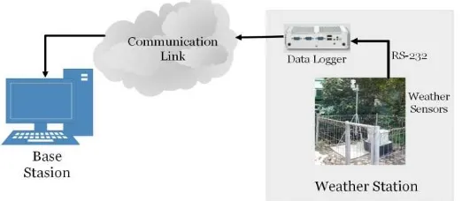
Weather monitoring system consists of a number of weather stations. One weather station has some weather sensors to measure and record weather parameters. Example of weather monitoring system configuration from one weather station can be seen on Figure 1. Weather parameters that measured in a weather station can be stored in a built in data logger or transmitted to a base station on remote location using a communication link. If the data are stored in a data logger, we can download them to a computer at a later time if we need for further processing [1].
There is a problem on this weather monitoring system. Data that are collected from a number of sensor nodes are so huge but the system constrained by limited power supply, memory, processing performance, and communication bandwidth. Three operations mainly responsible for energy consumption are sensing or sampling, computation, and communication [2]. When data transmitted on the network, energy consumption is dominated by radio communication. The energy consumption of radio communication is directly proportional to the number of bits of data that transmitted on the network [2]. Compression is a key to overcome this problem. The main objective of compression on this system is to reduce energy consumption by reducing number of bits that need to process and transmit on the system.
A large number of compression techniques have been proposed in the literatures [2, 3]. One of compression technique that interesting for many researchers nowadays is compressive sensing technique. Compressive sensing is new approach in signal processing, particularly for data acquisition [4]. On traditional data acquisition, signal can be reconstructed from the samples that are taking at a rate greater than Nyquist rate (2xfmax). On compressive sensing, a signal can be recovered from far fewer samples than Nyquist rate, as long as the signal is sparse or approximately sparse. It will only process the large coefficients and disregard the zero coefficients [6, 7]. This compression algorithm reduces the size of data sent and decreases the storage requirement of the system. This will also lessen the data transmission activity. This criteria is suitable for compression type that is needed in weather monitoring system.
On this paper, we evaluate compressive sensing algorithm for implementation on weather monitoring system. By using compressive sensing, number of measurement can be reduced and number of weather data that be collected become fewer, without sacrificing quality of the reconstructed signal. One of the problems on implementing CS on weather monitoring system is we don’t know the kind of representation basis under which the weather data be sparsely represented. A signal may not sparse in a particular domain (like time domain), but it can be sparse or compressible by transforming it to some suitable basis. There is no systematic way of selecting this kind of matrix. We can know the suitable basis by trials and experience [5]. On this paper, we evaluated performance of weather signal reconstructed using compressive sensing when representation basis is using Discrete Cosine Transform (DCT), Discrete Walsh Hadamard Transform (WHT), and Discrete Wavelet Transform (DWT). The objective is to select what kind of representation basis that make signal reconstruction error is minimum.
2. Compressive Sensing (CS)
CS is an alternative sampling theory which asserts that certain signal can be recovered from far fewer samples than Shannon-Nyquist sampling uses [3, 6]. According to Shannon – Nyquist theorem, the sampling rate must be at least twice the maximum frequency present in the signal [6, 8]. One of the key of the CS is that the signal is sparse or compressible [6]. A signal is called sparse if it has only a few significant components and a greater number of insignificant components. CS only focuses on large or non zero coefficient.
A discrete signal � of length n is said to be�-sparse, if � contains (at most) � nonzero entries with � ≪ �. A signal may not look sparse in a particular domain, but it can be sparse or compressible by transforming to some suitable basis, e.g., DCT, Fourier, or Wavelet basis. For many natural signals there are adequate bases and dictionaries in which signals of interest become sparse or approximately sparse. A signal is said to be compressible, if there is a basis in which the signal has approximately sparse representation [7]. Signal of interest � can be expressed in representation basis as:
�=Ψ� (1)
Where Ψ is transformation basis Ψ = { Ψ1, Ψ2, Ψ3,…, ΨN} and � is �-sparse vector, that represent projection coefficients of � on Ψ.
A main idea in the current CS theory is about how to acquire a signal. The acquisition of signal � of length � is done by measuring � projections of � onto sensing vectors { ����= 1,2, … ,� } [7]. On the matrix notation, the sensing process is described by [6-8]:
Where � ∈ �� is the signal to be sensed, and Φ is � ×� measurement matrix, and � ∈ �� is measurement vector.
A nonlinear algorithm is used in CS at receiver side to reconstruct original signal [3]. This nonlinear reconstruction algorithm requires knowledge of a representation basis Ψ. Measurement vector �, can be expressed in representation basis as:
�=ΦΨ� (3)
Θ=ΦΨ is � ×� dimensional reconstruction matrix, and we would have:
�=ΘS (4)
Reconstruction algorithm in CS is finding a sparse vector S satisfied (4) exactly or approximately with given � and Θ. � is an undetermined linear system who has more unknowns than equations. Finding a sparse solution of �=ΘS is an ill-posed problem [7]. Solution for this problem is done usually by minimizing l0, l1, or l2 norm over solution space. On this paper, we use l1 minimization to solve the problem. The compressive sensing algorithms that reconstruct the signal based on minimizing l1 referred to as Basis Pursuit (BP) [10]. By using l1 minimization or Basis Pursuit, signal can be exactly recovered from � measurements by solving a simple convex optimization problem through linear programming [10].
Minimize ‖�‖1; Subject to: ΦΨ�=� (5)
Once the solution l1 of (5) is found, reconstructed solution � my be expressed as:
�∗=Ψ�∗ (6)
3. Filtering Algorithms
On this research, we only focus on the monitoring of weather signal at a single location. We divided our simulation using two stages, signal acquisition and signal reconstruction.
3.1. Signal Acquisition
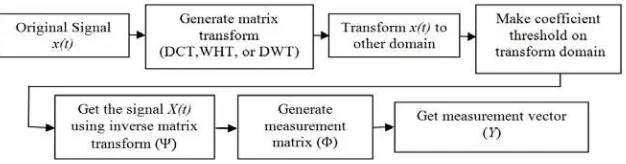
On this weather monitoring system, signal acquisition is a process for sampling weather signal that measure weather condition parameters on a region. From this signal acquisition stage, we will get measurement vector Y that will be used for signal reconstruction on the receiver side. The diagram on this signal acquisition stage can be seen on Figure 2 [7, 10].
Figure 2. Signal acquisition stage
Steps on this stage are [7, 10]:
1. Read the original signal �(�) from wireless weather monitoring system. 2. Generate matrix transform (DCT, WHT, or DWT) for sparsifying the signal. 3. Transform the signal using determined matrix transform.
4. Make coefficient thresholding on transform domain for sparsity enhancement [9]. Coefficients smaller than thresholding value (δ) set to zero.
6. Generate measurement matrix Φ (using random projection matrix), and then get the measurement vector �. This means that the measurement vector � was obtained by sampling signal � randomly.
3.2. Signal Reconstruction
The signal reconstruction is stage to construct the desired weather signal � from measurement vector �. Block diagram of this stage can be seen on Figure 3.
Figure 3. Signal reconstruction stage
Inputs for reconstruction algorithm are measurement vector �, measurement matrix (Φ), and representation basis (Ψ). The steps on this stage are:
1. Determine reconstruction matrix (Θ) from known Φ and Ψ.
2. Finding sparse vector (�) exactly or approximately with given � and Θ, using Basis Pursuit algorithm.
3. Reconstruct the weather signal � from given � and Ψ. .
4. Simulation Result
This section evaluates the effectiveness of CS implementation on weather monitoring system. For the evaluation we used real dataset without compression from wireless weather station that developed by Indonesian Institute of Sciences (LIPI). The first dataset is for humidity and the second one is for air temperature. Data taken on January 2015 in Bandung station. The data read once in every two minutes. On simulation, we used 2048 samples. Picture of the original signal samples can be seen on Figure 4.
(a) humidity (b) temperature
Figure 4. Original weather signal
Transform (DCT), Discrete Walsh Hadamard Transform (WHT), and Discrete Wavelet Transform (DWT). On wavelet transform, we used Daubechies d4 wavelet (db4 wavelet).
Results are presented on two parts. The first one presents the sparsity analysis of humidity and temperature data. This result is used for determining number of measurement or measurement matriks Φ. For sparsity enhancement, we used coefficient thresholding on transform domain. Thresholding value (δ) that is used on this simulation is 4. Sparsity (r) of the data can be seen on Table 1.
Table 1. Data sparsity using different basis Transforms Sparsity (r)
Humidity Temperature
DCT 99 20
WHT 141 37
DWT 111 25
From Table 1 we can see that DCT sparsifies the data better than other transforms. Number of measurement m is taken based on this sparsity analysis. From Table 1, maximum sparsity is 141. Based on previous research, number of measurement m must be higher or equal with 4 � [3, 7]. Based on this analysis, we take 600 as number of measurement.
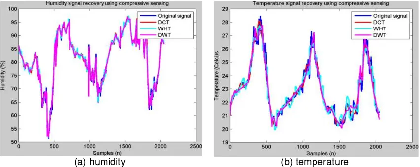
The second part of the results includes the performance of CS on recovering weather data using DCT, WHT and DWT as representation basis on sparsifiying weather signal. Recovered signal as results from simulation can be seen on Figure 5 and Figure 6. From the pictures, we can see that when comparing figures of the reconstructed signals with the original signal, the reconstructed signal is almost coincide with the original signal even though there are some errors. Its mean that we can recover signal with small number of measurement or sampling rate. How much error between original signal and reconstructed signal is tolerable depend on the purpose of the weather monitoring system, are the data critical or not.
(a) humidity (b) temperature
Figure 5. Reconstructed weather signal
The results on Figure 5 also show that three representation basis that used for sparsifying the signal give different performance on signal reconstruction. Error between original signal and reconstructed signal using compressive sensing algorithm was counted and we summarized it using Root Mean Square Error (RMSE) parameter.
����=1
��∑��=0(�(�))2, �ℎ����(�) =�(�)− �̂(�) (7)
Table 2. RMSE of signal reconstruction
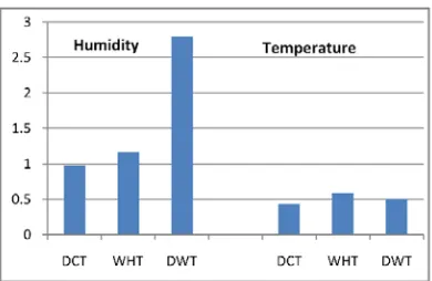
The results are also presented on a diagram on Figure 6. This figure shows that in case of humidity signal, signal reconstruction using DCT as representation basis shows the best performance, and DWT is the worst. On temperature signal, DCT also shows the best performance. On this temperature signal, WHT is the worst.
Figure 6. RMSE of signal reconstruction
By comparing the simulation results of humidity data and temperature data, we can see that the recovery of temperature data is much closer to the original signal or error recovery is smaller than humidity data. That is because representation basis using DCT is more suited for recovering signal like temperature signal. Even the reconstructed signal of humidity data cannot perfectly same with the original signal, the overall recovering is not bad.
6. Conclusion
In this paper, CS has implemented for data compression on weather monitoring system. This CS algorithm is used to reduce the number of samples required to recover the sampled signal and so reduce the energy consumption of the sensor in both sampling and transmission. We show CS can reduce the number of samples required to be taken in the weather monitoring system located in Bandung Indonesia. From simulation we proofed that DCT is the best transform coding to be implemented as representation basis for humidity and temperature data, as part of weather data.
References
[1] P Susmitha, G Sowmyabala. Design and Implementation of Weather Monitoring and Controlling System. International Journal of Computer Applications. 2014; 97(3): 19-22.
[2] MA Razzaque, Chris Bleakley, Simon Dobson. Compression in Wireless Sensor Networks: A Survey and Comparative Evaluation. ACM Transactions on Sensor Networks. 2013; 10(1).
[3] Saad Q, Rana MB, Wafa I, Muqaddasn N, Sungyoung Lee. Compressive Ssensing: From Theory to Applications, a Survey. Journal of Communications and Networks. 2013; 15(5): 443-456.
[4] Wen Yaw Chung, Jocelyn Flores Cillaverde. Implementation of Compressive Sensing Algorithm for
Wireless Ssensor Network Energy Conservation. International Electronic Conference on Sensor and
Applications. 2014.
[5] Xiaopei Wu, Mingyan Liu. In-situ Soil Moisture Sensing: Measurement Scheduling and Estimation
using Compressive Sensing. Proceedings of the 11th International Conference on Information
[6] Emmanuel Candès, Michael Wakin. An Introduction to Compressive Sampling. IEEE Signal
Processing Magazine. 2008; 25(2): 21-30.
[7] Wu-Sheng Lu. Compressive Sensing and Sparse Signal Processing. University of Victoria. Canada. 2010.
[8] Jianhua Zhou, Siwang Zhou, Qiang Fan. Mathematics Approach in Compressed Sensing.
Telkomnika. 2013; 11(9): 5435-5440.
[9] Ida W, Tati L, Andriyan BS, Hendrawan. Sparsity Properties of Compressive Video Sampling Generated by Coefficient Thresholding. Telkomnika. 2014; 12(4): 897-904.
[10] Shulin yan, Chao Wu, Wei Dai, Moustafa Ghanem, Yike Guo. Environmental Monitoring via
Compressive Sensing. Proceedings of the Sixth International Workshop on Knowledge Discovery from
Sensor Data. 2012: 61-68.