A LiDAR application to the study
of taxiway surface evenness and slope
M. Barbarella a, M. R. De Blasiis b, M. Fiani c,* , M. Santoni d
a
DICAM, Università di Bologna, Roma, Italy - [email protected] b
Dip. di Ingegneria, Università Roma TRE - Roma, Italy - [email protected] c
DICIV, Università di Salerno, Fisciano (SA), Italy - [email protected] d
GRS S.r.l., Roma, Italy - [email protected]
Commission VI, WG V/4
KEY WORDS: Experimental, Surface, Surveying, TLS, DEM/DTM, Accuracy, Estimation
ABSTRACT:
Pavement roughness evaluation of airport runways/taxiways and scheduling of maintenance operations should be done according to well-defined procedures. Survey of geometric features of airport pavements is performed to verify the flow of water from the surface and to assure a level of roughness that allows the airplane to maneuver in the safest and most comfortable conditions.
In particular the evaluation of longitudinal and transversal evenness of the runway and taxiway is carried out through topographic survey. The tachymetric survey has been carried out according to traditional topographic technique, which allows the evaluation of geometric position of isolated points with very high accuracy, but it is not very productive. Moreover it returns the pavement surface model through only few measured points. An alternative survey method, characterized by a good accuracy, high speed of acquisition and very high surveyed point density, is Terrestrial Laser Scanning (TLS), in static mode. In this paper we describe our experience aimed to validate the use of time-of-flight (TOF) TLS, based on a survey on a 200 m length segment of an international airport taxiway. From the acquired data we extracted the parameters of interest, especially the slope, and compared them with the values obtained from the traditional topographic survey. We also developed a proprietary software package to evaluate the slope and to analyze the statistical data. The software allows users to manage the flow of a semi-automatic calculation.
1. INTRODUCTION
The evaluation of airport pavement roughness needs a number of different measurements over the pavement. Implementation procedure, as well as typology and temporal interval of measures, are subjected to strict rules. Moreover the kind of instrumentations you need and the precision and the accuracy that such instruments must have are mandatory, in addition to the modality of data output. This system gives as advantage the chances to acquire a historical memory of the obtained survey results and as disadvantage the impossibility of making any protocol modification. Every variation has to be verified and certified and for this reason it is necessary to do studies and experimentation.
The survey of geometric characteristics of airport pavements is made to verify the flow of water from the surface and to guarantee a perfect surface regularity. The survey of pavement roughness characteristic is done in order to allow airplane maneuver execution in the safest condition.
ICAO (International Civil Aviation Organization) is the word wide organization that regulate civil aviation with the aim of standardize procedures for air traffic management, by issuing rules regarding also design and management of airport runway and taxiway (ICAO, 2013). International procedures in Italy are ratified by ENAC (Ente Nazionale per l’Aviazione Civile) the Italian civil aviation authority (ENAC, 2011). In particular, following the amendments n. 4-Annex 14 ICAO, concerning guidelines for design and management of airport infrastructure, it has been introduced the Safety Management System – SMS (ICAO, 2009).
According to ICAO the “Airport Certification”, which allows the airport workability, must contain, in addition to general information regarding the airport, operative procedures and
SMS organization and management (ADR, 2011).
According to ICAO organization, supervision and maintenance of the airport pavement, are based on the adoption of a Pavement Assessment Program (PAP). In order to minimize the interference with air traffic, PAP supports the adoption of non-destructive controls, which examine the pavement condition and the property of the material without causing any damage or modification to the pavement surface (ICAO, 2001).
The pavement performance model (Brockenbrough, 2004) supplies a global judgment of the pavement conditions, summarizing surface and structural characteristics: from the surface roughness to longitudinal and transversal evenness, from localized deformation to surface and structural cracking or skid resistance etc. Each type of road facilities, in relation to surface irregularities, requires a specific accurate rendering; it ranges from 0.5 mm to 50 m (PIARC, 1987).
Cracks and deformation resistances are considered the most important requirements with respect to the surface roughness. In particular the evaluation of the surface roughness has acquired a remarkable importance in control activities of airfield infrastructure and in monitoring pavement condition in order to verify the minimum international standard requirements. It is necessary to monitor surface evenness because they bring negative impact both on airplane and pavement itself. Pavement roughness directly influences airplane components during take off and, landing maneuvers, forcing higher stress and fatigue phenomenon which could lead to break mechanical parts and to reduce safety and comfort of airplane operation (cabin vibration, extreme g-force, loss of adherence, etc.).
operation safety: restricting adherence conditions and stressing the infrastructure in an unusual way and further supporting the degradation progress. Moreover, in aeronautical sector, the primary scope of airplane dampening system is to absorb the high stress generated during the landing phases; therefore the dampening system itself is calibrated to face this necessity. The instruments adopted for evaluating surface and structural characteristics of pavement present some characteristics that influence the measure. Choose an instrument rather than another primarily depends on the type of damage: GPR (Ground-penetrating radar) for the in situ evaluation of thickness and homogeneity of the layer, laser profilometer to define surface roughness of the pavement, skid testing for adherence condition and Falling Weight Deflectometer test for the bearing capacity (NCHRP, 2004).
Non Destructive Tests could present some disadvantage due to the methodology of the survey; for example the laser profilometer detects the profile of the pavement through a series of laser mounted over a longitudinal inertial staff strictly fixed to the vehicle. This kind of survey could have some limits depending on the motion dynamic (quarter car model for the determination of specific indicators) (Sayers, 1986).
A very viable and efficient survey method to evaluate road surface conditions is a Mobile Mapping System (MMS), (Schwarz and El-Sheimy, 2004) moving vehicle that continuously tracks its position via a navigation system (generally consisting of GPS, IMU and odometer) and contemporary gathers data on road surface conditions along its route with various onboard devices (namely laser scanner, high-resolution digital cameras, and often Ground Penetrating Radar and inertial profilometer) (Puente et al. 2013). A MMS allows the user to acquire data to be inserted into a pavement management system and to monitor the pavement condition (Riesner, 2014; Guan et al. 2014; Aoki et al., 2012; Dondi et al., 2011; ADS 2010). The very high productivity of MMS is not always accompanied by a high accuracy in the position of the measured points on the runway. Survey accuracy depends both on the measuring instruments (laser scanner, high-resolution cameras), and the navigation subsystem (generally consisting of GPS, IMU, odometer) that determines the position and attitude of the vehicle equipped with the instruments. Instruments placed on a tripod and fixed on a point, such as Total Station, Levels and Terrestrial Laser Scanners give greater guarantees of accuracy.
Tachymetric survey aims to verify the transversal and longitudinal slope of the runway, taxiway and apron area, allowing the evaluation of the roughness parameter. Generally this kind of survey is carried out with a high precision robotic total station with a 360° prism mounted over a pole carried over the point to be measured. Moreover height is measured with high precision level by the Invar stadia. Therefore through the traditional topographic survey it is possible to measure coordinates of the whole pavement through spot points. Although the tachymetric survey is characterized by high precision, the use of total station has a high limit due to the point density, equal to the spatial continuity of the acquired information (usually the point are taken with a grid 10 m x 10 m). This limit brings to the impossibility of evaluating any punctually deterioration over the pavement, like fracture and rutting, in addition to the detection of localized roughness discrepancies. The total station allows the user to obtain profile of the runway with the precision requested for the evaluation of the airport parameter. Once the survey is carried out, it is possible to create a Digital Elevation Model (DEM), from which transversal and longitudinal profiles of the centerline are extracted on the area on which air traffic tends to touch down. It could be possible to use terrestrial laser scanning surveys
instead of tachymetric surveys. Considering the performances of the most recent instrumentation in terms of range, accuracy, point density and acquisition speed, it should be interesting to evaluate the on-field performances. The field test site has a length of about 200 m. The elaboration of the measures allows the evaluation of the transversal and longitudinal slope of the taxiway and the comparison with the result of the tachymetric survey. The aim of our experimentation is the definition of operative and computational procedures together with the evaluation of the results accuracy. Moreover the tests aim to understand if the laser scanning survey could compete, in economic terms, with the traditional method of survey. The survey of the pavement surface has been performed through a series of equally spaced laser scanner stations localized over the centerline of the taxiway, so to acquire transversal and longitudinal slope. These parameters must satisfy the rigorous norms defined by airport Authorities. Acquisition specifications of the point clouds and data elaboration have concerned the modelling, in terms of transversal and longitudinal profile, in order to satisfy the condition sets out by ICAO and ENAC.
2. METHODS
The use of TLS set up over a series of points allows, in theoretical terms, to achieve sufficient accuracy for the survey of the taxiway, aimed to define the surface geometry. The object of the test is verifying, experimentally, if it is possible to reach the expectations and to compare the survey and elaboration difficulties, related to traditional methods.
For the evaluation of the geometry of the taxiway it is currently used both high precision Level, to assess the materialized points height with benchmark, and Total Station (TS), for the survey of profile distributed regularly along the runway. Through the elaboration of the profile points it’s possible to evaluate transversal and longitudinal slope of the pavement surface. TS is localized over station points and the reflector prisms stand over survey points with a constant step (in the order of some meters). Survey distances could be even higher, without having significant accuracy loss, for the evaluation of angles and distances, and consequently in the measure of the ground point coordinates when the prisms are set up.
The TLS, similarly, is set up over points on the centerline but it directly measures points belonging to the pavement, with a sampling rate in zenith and azimuth angles defined by the operator. The results of the survey are many point clouds on the pavement with very high density, even if variable with the distance from the instrument to the points. The greater the distance, the lowest the incident angle of the laser ray over the pavement, the greatest the contact patch and the lowest the energy reflected back to the instrument.
reference System is not mandatory since you can geo-referencing the whole cloud later. In our case the geogeo-referencing of the TLS survey in the Airport Geographic System is not useless. To do this, you can survey the target positions with traditional topographic technique, using GNSS/GPS receiver in RTK mode (or NRTK if possible); the master station can be put directly over airport frame points. All the commercially available software packages for analyzing laser data allow the georeferencing over a known set of points having a different reference system. The development of a GRID DEM starting from a points cloud is based on the choice of the interpolation algorithm and of the distances of the points over the grid node (Kraus and Pfeifer, 2001; Vosselman and Sithole, 2004; Pfeifer and Mandlburger, 2009). The surface roughness simplifies the choice, however it is possible to select between different methods (Inverse distance to a power, Kriging, Radial Basis Function, etc.).
In order to establish the final result we usedthe same approach we adopted in a different setting (Barbarella et al., 2013), i.e. we extracted a sub-sample of point clouds (1%) and we built a DEM, utilizing a number of algorithms, and we evaluated statistical parameters, related to the variance of the sub-sample compared with the DEM in the same planimetric position. The test underlines a substantially equivalence between the algorithms above mentioned. In this experiment we chose Inverse Distance to a Power (2 degree). The obtained DEM allows the reconstruction (numerical) of the runway surface; starting from that, it is possible to extract any section or profile you need.
We used the following method for the automatic choice of significant sections and the extraction of the corresponding profile. First we surveyed the planimetric position of the centreline, with GPS or TS; then we calculated the extremes of line segments of set width, orthogonal to the axis, at intervals along the axis line also chosen by the operator; thereafter we interpolated the DEM along those sections, obtaining the profiles, i.e. a number of sequences of pairs of values, progressive distances and interpolated height.
The knowledge of the centerline position allows the user to divide the cross-section profiles in two sub-systems, one at right and the other at left of the centerline so to calculate the slope values of each one. For the estimation of the slope we calculated the line that better interpolate all points of every segment, using the least squares method. The angular coefficient of the line is the slope of the section.
In order to perform this task we wrote a specific software code in Matlab. The analysis of the profile, particularly when it is located near the edge of the grid, highlights some noise due to the objects that might be on the surface, such as cylindrical tie-points used for the scan co-registration and some parts of the surface that deviate from the linear trend of the pavement profile (for example the counter-slope).
It is necessary to identify the limits of a single slope side and isolate the two sets of profile points in order to analyze only one straight transversal profile and evaluate the slope. For the previous purpose, the software allows the user to:
- represent every elevation profile with lines that symbolize centreline and edge section position;
- accept or modify the edge position of the section through the cursor movement, in order to define two straight sides; - interpolate the points that belong to each side with the least
square method, in order to evaluate the linear regression parameter of best fit; the gradient coefficient is the slope of every side.
For the evaluation of longitudinal slope it is possible to create parallel lines to the centerline, e.g. located 3, 6 and 9 meters away from the axis and to evaluate the profile along that
alignments. It is necessary to study significant value of that slope to consider all the parts of the longitudinal profiles, as well as the norms requires. Eventually the profiles extracted from the DEM could be compared with the ones obtained with the TS; it is also possible to compare the slope values of the straight sections obtained on the same part with both surveying methods.
3. TEST SURVEY AND DATA ELABORATION
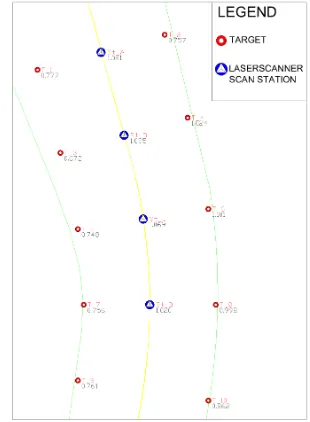
The survey area lies over a part of about 200 m of a taxiway of an international airport. Pavement survey was done through the TLS, time of flight technology, Riegl VZ-400. The field campaign has been carried out at night times, when airplane traffic was reduced and the survey does not create problems to airplane circulation. Point clouds were acquired from four stations, localized over the centerline with a sign on the surface, spaced each other’s 30 m. The instrument was set up over a strong tripod, equipped with a central telescopic axle. Spherical targets with radius of 0.15 m were mounted over tripods set up over points materialized with topographic nails, fixed inside the pavement. Each one of the four stations contain 4 to 6 targets, localized axle, which allows the raising of the instrument to 2.2 m. In order to georeferencing the data we used fifteen targets sphere shaped, placed close to the edge of the pavement away 20-40 m from the TLS point stations. The position of the topographic nails was measured with GPS in RTK mode. GPS master antenna was mounted over a tripod near the survey area, while antennas of rover receivers were mounted over poles. The transmission of corrective data was done via radio modem. The transformation of the point coordinates in the cartographic airport system (the Italian national system Gauss-Boaga) was done though the GPS vertexes, linked to four points of known coordinates. During the field campaign we also made a high precision geometric levelling, to assign the orthometric height to the vertexes measured with GPS, starting from a benchmark located inside the airport. Figure 1 shows the TLS survey scheme.
Figure 1. TLS survey scheme carryed out on the taxiway
sphere starting from the point cloud. Every point cloud was co-registrated with the others and the resultant points cloud was geo-referenced through the target coordinates.
The geo-referenced global cloud was divided in four parts, in order to reduce the file dimension. Each file contains the points of the initial cloud, which keeps the new acquired position. We used the algorithm “Inverse Distance to a Power” (2 degree) for the point cloud interpolation onto the DEM GRID. The grid step was fixed at 2.5 cm, which is the mean distance of the points at 25 m far away from the TLS stations.
The developed software package permits to section the DEM along lines orthogonal to the centerline, close as you want, but of fixed length, in order to extract a number of transversal or longitudinal profiles. Eventually the program gives in output the slope values by calculating the straight-line parameters that better interpolate the profiles. The taxiway part surveyed with TLS has been surveyed the previous day with tachymetric survey system, using a Total Station Topcon GPT-9001A and a high precision level Leica DNAA03.
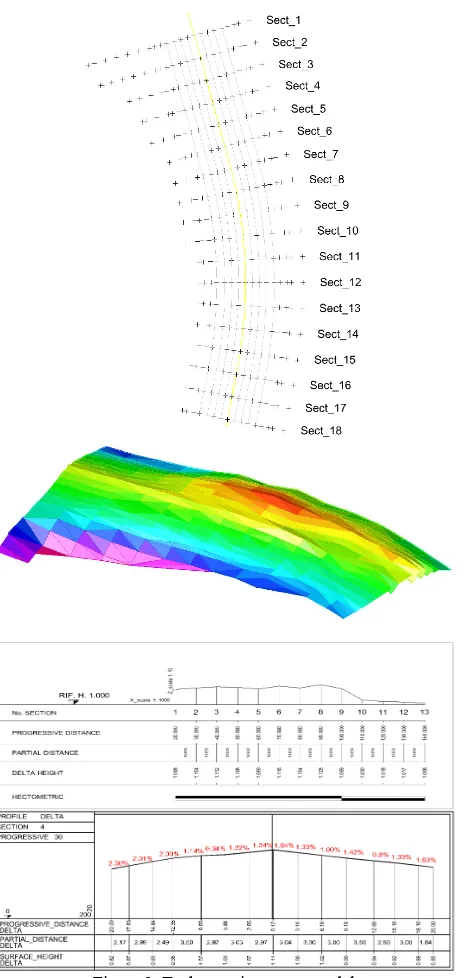
Figure 2. Tachymetric survey model
The TS was settled up over a number of vertexes; some points along both the centerline and parallel lines at 3, 6, 9, 15 m far away and at the edges were acquired. The longitudinal step of the acquired points was 10 m. The point grid of the survey is shown in figure 2.The same figure shows the DEM build from the ground surveyed points and a transversal and longitudinal standard profile, extracted from DEM. The knowledge of the planimetric coordinates of the end sections allows us to define the correspondent profile of the DEM that is derived from the point clouds. Moreover, we measured with GPS the position of the points where we located the target during the survey (figure 1).
4. RESULTS
The results of the elaboration of TLS data consists in a series of transversal and longitudinal profiles of the runway segment, which can be used to obtain information about the pavement condition and its correspondence to specifications.
The implemented software allows us to obtain any number of profiles and each profile consists in any number of points, in line with the input data density and the DEM grid. In our experiment we realized transversal and longitudinal profiles with variable steps, according to the product to analyze. We extracted profiles to make a comparison between the TLS and the tachymetric survey along the same sections, every 10 m in transversal direction, with point located along both the centerline and other lines at 3-6-9 meters far away, on the left and right side.
4.1 Transversal and longitudinal profiles of the runway
We built transversal profiles with very high point density, up to 2.5 cm, to evaluate the irregularities. These profiles include both a straight segment with two different slopes, and a curved segment with single slope. Interim profile joins curved and straight segments. Figure 3 shows the 40 profiles extracted, orthogonal to the axle along the section, generated every 5 m, with a length of 30 m (15 m on the left and 15 on the right). The high density of the point cloud along the profile (one every 2.5 cm) allows us to observe high frequencies and irregularities. We can clearly see the shape variation in the pavement survey and the slope differences in the curve for the water flow.
Figure 4 shows the longitudinal profile obtained along both the centerline and the other parallel alignments. In better detail, the chosen alignments are at 3-6-9 meters distant from the axle because these are the localizations of the main gears of the airplane. Also these profiles consist of points profiles consist of points that are 2.5 cm far from each other. The high point density allow to obtain high detailed profile, in accordance with the point cloud density; that allows the user to know the pavement conditions and if any macro damage is present.
Figure 3. Transversal profiles every 5 m along the taxiway 0,8
0,9 1 1,1 1,2 1,3
0 5 10 15 20 25 30
distance (m)
h
e
ig
h
t
(m
Figure 4. Axle and ±3, ±6, ±9 alignments longitudinal profile
4.2 Traditional survey comparing
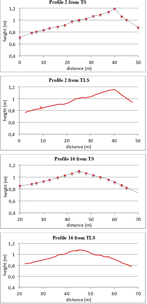
The transversal profiles determined by tachymetric survey over the tested part of the runway are 17 in total, one every 10 m of length. Along these profiles, the ground surveyed points are located in axle, edge runway and at ±3, ±6, ±9, ±15 meters far away, both on the right and the left side (see figure 2). The points extracted from TLS’s DEM, used for the comparison, are located in correspondence with the same section positions. Theoretically the traditional survey with TS along defined alignments allows the user to immediately obtain measures of profile and slope and also to build a DEM in order to have geometrical information also over portions that are not directly surveyed. However the points ground surveyed with TS are spaced about ten meters and they do not allow us to do an accurate analysis of the surface. Figure 5 shows two standard profiles, obtained both with the tachymetric survey and TLS; profile n. 2 corresponds to a portion of the taxiway in curve whike the n. 16 to a straight part. It clearly shows how the highly dense point cloud of the TLS survey allows the user to have a continuous visualization of the transversal profile in order to better analyze the very high frequencies that are not visible with the traditional survey that is discrete by its nature. We calculated, for all the 17 transversal profiles, the height
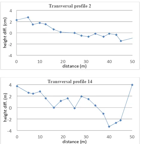
differences between the points surveyed with traditional topographic method and the correspondent ones (same planimetric coordinate) extractd from the TLS’s DEM. We considered only a central segment of the runway with size equal to 50 m, 25 m on the left and 25 on the right of the centerline. Figure 6 shows the differences between the two sections, n. 2 and n. 14; figure 7 shows the difference mean for the 17 sections; figure 8 shows the differences between the longitudinal profiles.
The height differences between the two different types of survey are significant, estimated in the range of 1 to 2 cm with some large fluctuations. We do not consider a priori that a traditional tachymetric survey represents a more precise reference even though the measured differences are considerable. We hold that, to make a proper quality control of a DEM, it’s necessary to perform a tachymetric survey according to some specifications.
Figure 5. Standard profile surveyed with tachymetric and TLS surveying method
0,4 0,6 0,8 1 1,2
0 10 20 30 40 50
h
e
ig
h
t
(m
)
distance (m)
Profile 2 from TS
0,4 0,6 0,8 1 1,2
0 10 20 30 40 50
h
e
ig
h
t
(m
)
distance (m)
Profile 2 from TLS
0,4 0,6 0,8 1 1,2
20 30 40 50 60 70
h
e
ig
h
t
(m
)
distance (m)
Profile 16 from TS
0,4 0,6 0,8 1 1,2
20 30 40 50 60 70
h
e
ig
h
t
(m
)
distance (m)
Figure 6. Differences between transversal profiles obtained with the two different survey methods
Figure 7. Mean of the height differences for the 17 profiles
Figure 8. Differences between longitudinal profiles obtained with the two different survey methods
4.3 Slope and residual value profiles computation
Cross slopes and any local deviation from the straight interpolating line are two many important elements that user must keep under control for the runway analysis, since they are regulated by norms. If the values mentioned above are not included into the range of permitted value, a maintenance intervention is needed.
As shown previously, the profiles acquired from the DEM describe with high detail the cross-slope section trend and show the differences from the linear trends in some parts. It is therefore necessary to quantify the characteristics of the pavement / sections. Figure 3 shows us how difficult is to
identify the two extreme points that delimit a part that can be considered straight. In order to evaluate the two different slopes we identified, for every sections, the extreme points that could be considered straight for every slopes, in order to leave out of the interval the effects of the edges and counter-slope. These effects are visible in figure 3 and they are outside the runway part where the gear passes. In order to evaluate the cross slope for every portion we considered the points that define the altimetric profile, both for the left {d1i, z1i; i=1,2..,n1} and right slopes {d2i, z2i; i=1,2..,n2}, where d indicates the progressive distances along the profile and z indicates the DEM interpolated elevation.
For every sample, in accordance with the Least Square criteria, we consider the linear best fit of the sample:
�=�+��
where b is the searched gradient.
We obtained the parameter estimation of the straight line from the mathematical system solution; in better detail, the slope value is:
We assumed for the whole factor the same weight, pi = 1 Finally, we calculated the standard deviation of slope with the following:
It can be observed how the “sb” value depends strongly on the sample size “n”. It does not depend on the direct measure of the height but derives from the DEM interpolation, according to an arbitrary step chosen by the user: greater is the “n” value lower is standard deviation. The statistical model we chose (weight matrix W diagonal) did not take into account the correlation between the height data.
We preferred to assume as dispersion parameter (as indicator of the deviation of the height from the linear trend), the quantity that appears to be less sensitive to the sample size. Figure 9 shows the slope value estimated on the left part of the taxiway on the cross sections orthogonal to the axle, spaced 5 m from each other.
Figure 9. Slope of the left part of the taxiway
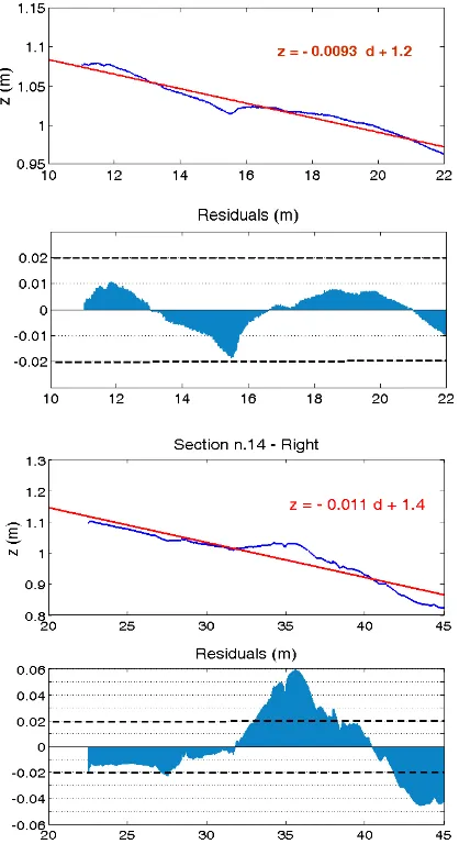
The chart allows the user estimate that slope values are inside the range value proposed by the regulations. It could be of same interest to evaluate the deviation of the profiles from the interpolating lines for every single slopes: TLS points density along the profile allows us to made this evaluation, by calculating the residual of the fit:
The residual graph allows us to visualize the right side of the pavement as showed in figure 10. This type of visualization underlines the maximum values of the residuals and allows us to localize any portion of pavement that deviate from the trend for more than a certain limit value. For the section n.16, deviation from the trend is higher than 1 cm only for a short part, while for the subsequent profiles the deviation exceeds 2 cm for several meters. The developed software makes the localization of the section with respect to the absolute system possible so that the area where the deviation reaches the maximun values can be easily localized. It also calculates some statistical parameter: mean and median of residuals, etc. and the length of the track where the residual values exceed a limit value fixed by the user, too. As we said, the interpolated height values of the DEM differ from the tachymetric ones, so it’s quite obvious that the calculated slopes are different. Figure 11 shows profile slope values, obtained from the field survey and from the DEM. In some areas the differences are large.
Figure 10. Right slope for two examples of cross-sections; slope of the profile and residuals with respect to the interpolating line
Figure 11. Slope profiles surveyed by TLS and TS
There is a relationship between the required surface qualities and the range of irregularities that influence them. In particular the irregularity called “megatexture”, situated between “macrotexture” (roughness) and “evenness”, are the most important factor for the evaluation of pools (water flow), noise, driving resistance, etc.
The presence of microtextures and macrotextures is necessary to guarantee tire friction; on the contrary the presence of megatexture and unevenness is undesirable. These two fields of irregularities are approximately divided at about 50mm wavelength, which is approximately the average diameter of the surface of tire/pavement contact.
For the airport pavements the most important requirements is the correct evenness in the field of megatexture to avoid pools, to do not increase stress and wear of aircraft component and other factors that may impair the safe operation of the aircraft (FAA, 2009). We develop another Matlab code to evaluate the degree of regularity of a pavement that allows us to calculate the interpolated plan of the point clouds measured through TLS. The evaluations are carried out dividing the taxiway in parts of 3 m width, for every side. This allows us to evaluate strip above and below the average level plan and highlight the evenness degree of that strip (Figure 12).
Figure 12. Taxiway strip profile (3m width side) and interpolated plan. Left panel: section; right panel: axonometric
view
6. DISCUSSION AND CONCLUSIONS
The result obtained from tests justifies the interest around the application of TLS system for both the control of the performance of the road surface and the construction and management of the pavement. The speed, the easy use and the high level of accuracy obtained for the pavement survey, allows us to use this technique for controlling the quality during the construction phase. Moreover the obtained results underline the reliability of the measure opposed to the traditional techniques. This characteristic could be more appreciated in airport environment, both for the difficulties of air traffic and for the high level of accuracy required for the measure.
The amount of data acquired in a very short time with TLS causes problem for the management of the data itself, but they
ˆ
ˆ
i i
i
v
=
z
−
a
−
b d
0,8 1,2 1,6 2,0
0 50 100 150 200
sl
o
p
e
(
%
)
distance (m)
could be overtaken with commercial software packages. We choose to develop specific codes for the pavement study (both for a qualitative and quantitative point of view) that allow us to obtain profiles in a semi-automatic way along section orthogonal or parallel to the centerline. Moreover the software used for the transversal profile produces directly the slope value for both gradients with the Least Square procedure.
The slopes could be obtained with the same criteria also for single profiles surveyed with the TS, but their alignment has to be prior fixed and they are obviously much less numerous. Moreover the points surveyed with the two technologies are numerically not comparable. Once the DEM from TLS is realized, you can at any time thereafter have a very detailed description of the pavement, which could be queried in every moment, anywhere.
The height comparison between the directly surveyed TS points and the ones interpolated from the DEM by TLS data shows appreciable differences, which sometimes become significant. It must be noticed that the density of the DEM grid (unlike to that obtainable by TS) allows the user to locate parts of the profiles where the surface deviates significantly from the linear linear trend of the pavement; a specific code is able to quantify entity and depth of the differences. The study has therefore highlighted the increased reliability of procedures aimed to verifying the acceptability of the structural characteristics of a runway.
Where the control could not be done on discrete elements and it’s necessary to evaluate the continuity of the surface, the TLS technique could increase significantly the reliability of the measure. It would be appropriate to deepen our study, also doing more experimental tests, in order to determine what level of accuracy the TLS static survey allows the user to achieve; critical elements are of course the spacing between the laser stations, the accuracy in geo-referencing the clouds, the choice of the interpolator and the grid step of DEM.
We found useful, for the evaluation of evenness, divide pavement in strips with a limited number of points and detect any portion of surface in which the residuals from the best-fit plane are larger than a given threshold value.
REFERENCES
ADR, 2011. Airport Pavement Management System. Second Edition. Aeroporti di Roma.
Aerial Data Service, 2010. Meacham International Airport (KFTW). Runway 17/35: Mobile Mapping Runway Profile Demonstration.www.aerialdata.com/Meacham_LiDAR_Collect _Report.pdf.
Aoki, K., Yamamoto, K., Shimamura, H., 2012. Evaluation model for pavement surface distress on 3D point clouds from mobile mapping system. In: The International Archives of the Photogrammetry, Remote Sensing and Spatial Information Sciences, Vol. XXXIX, Part B3, pp. 87-90.
Barbarella, M., Fiani, M., Lugli, A., 2013. Landslide monitoring using multitemporal terrestrial laser scanning for ground displacement analysis. Geomatics, Natural Hazards and Risk, 11(2013), pp. 1-21.
Brockenbrough, R.L., 2012. Highway Engineering Handbook. Building and rehabilitating the infrastructure, 3th Edition. McGraw-Hill, New York.
Dondi G., Barbarella M., Sangiorgi C., Lantieri C., De Marco L., 2011. A semi-authomatic methodology to identify defects on a road surface. In: ICSDC 2011 Integrating Sustainability
Practices in the Construction Industry, KANSAS CITY, Oswald Chong and Christopher Hermreck, 2011, pp. 704-7011.
ENAC, 2011. Regolamento per la Costruzione e l’Esercizio degli Aeroporti. Amend 8 ed. 2 del 2003 – Ente Nazionale Aviazione Civile.
FAA, 2009. Guidelines and Procedures for Measuring Airfield Pavement Roughness. AC 150/5380-9, Federal Aviation Administration, Washington D.C.
Guan H., Li J., Yu Y., Wang, C., Chapman M., Yang, B., 2014. Using mobile laser scanning data for automated extraction of road Markings. ISPRS Journal of Photogrammetry and Remote Sensing, 87(2014), pp. 93-107.
ICAO, 2001. Doc 9774 Manual of certification of aerodromes. First Edition. International Civil Aviation Organization, Montréal, Quebec, Canada.
ICAO, 2009. Doc 9859 Safety Management Manual. Second Edition International Civil Aviation Organization, Montréal, Quebec, Canada.
ICAO, 2013. Annex 14 to the Convention on International Civil Aviation. Aerodromes Vol.1 Aerodrome Design and Operation - Sixth Edition. International Civil Aviation Organization, Montréal, Quebec, Canada.
Kraus, K., Pfeifer, N., 2001. Advanced DTM generation from LIDAR data. In: International Archives of the Photogrammetry, Remote Sensing and Spatial Information Sciences, Vol. XXXIV Part 3/W4, pp. 23-30.
NCHRP, 2004. The Mechanistic-Empirical Design Guide Part 2. NCHRP Transportation Research Board of The National Academies.
Pfeifer, N., Mandlburger. G., 2009. LiDAR Data Filtering and DTM Generation. In: Topographic laser ranging and scanning. Principles and Processing, Ji Shan and Charles K. Toth (Eds.), Taylor and Francis.
PIARC, 1987. Report of the Committee on Surface Characteristics. Proceedings of the 18th World Road Congress, Brussels, Belgium.
Puente I., Solla, M. González-Jorge, H., Ariasa, P., 2013. Validation of mobile LiDAR surveying for measuring pavement layer thicknesses and volumes. NDT & E International, Vol. 60, December 2013, pp. 70-76.
Riesner, E., 2014. Modern Airfield Pavement Management Strategies. In: The 2014 Airports Conference, March 3–5, 2014, Hershey, Pennsylvania.
Sayers, M.W., 1986. Guidelines for conducting and calibrating road roughness measurement, World Bank Technical Paper n. 46. Washington D.C.
Schwarz K.P., El-Sheimy N., 2004. Mobile Mapping Systems – State of The Art and Future Trends. In: International Archives of the Photogrammetry, Remote Sensing and Spatial Information Sciences, Vol. 35, Part 5, pp. 759-768.