Journal of Econometrics 95 (2000) 25}56
Estimation of a censored regression panel data
model using conditional moment restrictions
e$ciently
Erwin Charlier
!
,
"
,
*, Bertrand Melenberg
!
, Arthur van Soest
!
!Tilburg University, Department of Econometrics and CentER, P.O. Box 90153, 5000 LE, Tilburg, The Netherlands
"ABP Investments, Fixed Income Europe, P.O. Box 2889, 6401 DJ, Heerlen, The Netherlands
Received 1 November 1995; received in revised form 1 January 1999; accepted 1 April 1999
Abstract
HonoreH has introduced a semiparametric estimator for the censored regression panel data model with "xed individual e!ects. Newey has shown how to obtain e$cient estimators under a given conditional moment restriction. We apply Newey's approach to obtain a two-step GMM estimator which is more e$cient than the HonoreH estimator. We compare this estimator to the HonoreH estimator and to parametric estimators including Chamberlain's quasi-"xed e!ects estimator in a Monte Carlo experiment. We also extend the HonoreH estimator and the two-step GMM estimator to the case of a balanced or unbalanced panel of more than two waves. We apply the estimators to an empirical example concerning earnings of married females, using data from the Dutch Socio-Economic Panel. ( 2000 Elsevier Science S.A. All rights reserved.
JEL classixcation: C14; C23; C24
Keywords: Panel data; Censored regression; Semiparametric e$ciency; Unbalanced panel
*Corresponding author. Tel.:#31-13-66-91-11; fax:#31-13-66-30-72. E-mail address:[email protected] (E. Charlier)
1. Introduction
This paper considers estimation of the censored regression panel data model with individual e!ects. This model has important applications in micro-econometrics. The seminal example is the labor supply model of Heckman and MaCurdy (1980), where nonparticipation leads to censoring at zero, and where the individual e!ects have a clear economic interpretation in a life cycle context. Other examples are Udry (1995), who analyzes grain sales and purchases of rural households in Nigeria, and Alderman et al. (1995) and Udry (1996), who analyze various types of labour inputs and manure input in agricultural production.
Two types of estimators for this model can be distinguished. Estimators which require a parametric speci"cation of the model are discussed by Chamberlain (1984). These models have the advantage that not only the parameters can be estimated, but also quantities such as marginal e!ects of covariates on the observed censored variable, which may be more interesting than the parameters themselves from a policy point of view. On the other hand, they have the drawback that estimates of the parameters of such e!ects will, in general, be asymptotically biased if the parametric model is misspeci"ed. To overcome this problem, HonoreH (1992) has introduced a semiparametric version of the model, which avoids assumptions on the distributions of individual e!ects or error terms. He derives consistent estimators for the parameters of this model, but does not address estimation of the marginal e!ects.
In this paper, we introduce a new semiparametric estimator, which aims at improving the e$ciency of one of the HonoreH (1992) estimators. HonoreH 's estimator is based upon (unconditional) moment restrictions derived from a conditional moment restriction. Following Newey (1993), we nonparametri-cally estimate the optimal moment restrictions for HonoreH 's conditional moment restriction, and construct a two-step GMM estimator which will be asymptotically more e$cient than the HonoreH estimator. Like HonoreH 's es-timator, our estimator is easy to compute. It is e$cient in the class of estimators based upon the given conditional moment restriction, but does not attain the semiparametric e$ciency bound for HonoreH 's semiparametric model, since this model leads to many more conditional moment restrictions, which our es-timator does not exploit.
using data drawn from the Dutch Socio-Economic Panel (SEP). Stoker (1992) uses earnings of married females as the prototype example of a censored regression model in a cross-section framework. Since unsystematic earnings variations mainly re#ect changes in labour supply, it is natural to add "xed e!ects (Heckman and MaCurdy, 1980).
The remainder of the paper is structured as follows. In Section 2, we present the model and discuss merits and drawbacks of existing parametric and semiparametric estimators. Section 3 introduces our two step GMM estimator and its properties for the case of two time periods. In Section 4, we compare semiparametric and parametric estimators in a Monte Carlo experiment. Sec-tion 5 considers the empirical applicaSec-tion for two time periods. In SecSec-tion 6, the GMM-estimator is extended to panel data with more than two waves, either balanced or unbalanced. In Section 7, it is applied to the same empirical example, using"ve waves of SEP data, from 1984 to 1988. This section also presents the economic interpretation of the results. Section 8 concludes.
2. Parametric and semiparametric models and estimators
The censored regression model for panel data with individual e!ects is given by
yH
it"ai#b@0xit#uit, i"1,2,N,t"1,2,¹,
y
it"maxM0,yHitN.
Hereidenotes the individual andtis the time period,y*
itis a latent variable,yitis
the observed dependent variable,x
itis a vector of covariates,aiis the individual
e!ect, u
it is an error term and b0 is a vector of unknown parameters to be
estimated. We observe (y
it,xit). We are interested in asymptotic results for
NPR, but for"xed¹. We assume independence across individuals, but not necessarily over time. We discuss various models with di!erent assumptions and corresponding estimators.
In models with random e!ects, a
i is assumed to be independent of
x
i"(x@i1,2,x@iT)@. Several parametric random e!ects models and corresponding
estimators for b0 have been proposed in the literature. For example,
ai&N(0,p2a) andu
i"(ui1,2,uiT)@&N(0,R), with R"p2uITandITthe¹]¹
identity matrix, yields the speci"cation of equicorrelation of Heckman and Willis (1976). Here Maximum Likelihood (ML) can be applied. This requires numerical integration in one dimension. If milder restrictions onRare imposed, estimators can be based on¹!1 dimensional numerical integration or simula-tion (such as simulated ML or simulated moments; see Gourieroux and Monfort, 1993).
If the assumptions on the distributions of error terms and individual e!ects are satis"ed, the estimators are consistent and asymptotically normal. If the assumptions of normality of (u
i,ai) or independence between (ui,ai) and xiare
not satis"ed, the estimators will generally be inconsistent (see, for example, Arabmazar and Schmidt, 1981,1982).
Parametric models with"xed e!ects can be divided into two categories. In the
"rst, no restrictions on the distribution ofa
iconditional onxiare imposed. The
a
iare then usually considered as nuisance parameters. In the second category,
some restrictions on the distribution ofa
iare imposed, which do not exclude
dependence betweena
iandxi.1
In models in the "rst category, it is usually assumed that u
it,
i"1,2,N,t"1,2,¹, are i.i.d. and independent ofxi. Since theaiare
para-meters, models in this category su!er from the incidental parameter problem, see Neyman and Scott (1948). ML estimates will generally be inconsistent. For a speci"c distribution of the u
it, b0 could be estimated up to scale using
Chamberlain's conditional logit estimator, but this approach does not work in general.
An example of a model in the second category is given by Chamberlain (1984). It assumes thata
i"a@0xi#wi, witha0an unknown vector of (nuisance)
para-meters, w
i&N(0,p2w), ui&N(0,R) without restrictions on R, and wi,ui and
x
i independent. Chamberlain proposes a two stage procedure to estimate b0.
First the reduced-form model for each cross-section is estimated, ignoring restrictions on the parameters across time. The second step is minimum dis-tance, to take account of these restrictions. This model allows for a speci"c form of correlation betweenai andx
i, but it retains the assumption of normality of
w
iandui. Fora0"0, it simpli"es to a random e!ects model.
The main goal of semiparametric estimation is to avoid the distributional and independence assumptions discussed above, and to construct estimators of
b0which are consistent under more general assumptions. HonoreH (1992) derives various semiparametric estimators for the case¹"2. He provides two repres-entations of the identi"cation assumption. We use the representation stated in HonoreH (1992, Assumption E.3, footnote 6). The starting point is the following basic assumption (with the subscriptisuppressed from now on):
(A1) (Conditional exchangeability assumption). The distribution of (u
1,u2), conditional on (a,x1,x2), is absolutely
con-tinuous and u
1 and u2 are conditionally interchangeable (i.e., have
conditional density f, with f(u
1,u2Da,x1,x2)"f(u2,u1Da,x1,x2) for all
(u
1,u2) and (a,x1,x2)).
Assumption (A1) allows for nonnormality and dependence between the errors and (a,x
1,x2), and imposes no restrictions on the distribution of a
conditional on (x
1,x2). In this sense it is more general than the assumptions
needed by Chamberlain (1984). On the other hand, the Chamberlain (1984) model is not fully nested in that of HonoreH (1992), since Chamberlain (1984) does not impose that the conditional distributions of u
1 and u2 have the same
variance.
HonoreH derives two conditional moment restrictions (CMRs) from (A1). He then constructs unconditional moment restrictions (UMRs) from these CMRs. The value of the (generic) parameter vector b which satis"es the empirical counterpart of these UMRs provides a consistent estimator ofb0. The UMRs are chosen in such a way that these empirical counterparts of the UMRs are the
"rst-order conditions of minimizing a strictly convex objective function with
respect tob, implying that the estimates are easy to compute with a local search algorithm.
Each CMR yields its own estimator forb0; HonoreH does not combine the two CMRs. The two estimators share the property that, in the UMRs or the objective function, (b,x
1,x2) appears only as b@(x1!x2). This implies that
estimation hinges on variation in*x"x
1!x2. The coe$cients of
time-invari-ant regressors are not identi"ed.
We will use HonoreH 's second estimator, for which the corresponding objective function is everywhere continuously di!erentiable and twice di!erentiable in all but a"nite number of points (the UMRs are given in (2.5) in HonoreH (1992)). This makes it straightforward to derive the limit distribution of this estimator and to estimate its covariance matrix. The corresponding CMR will be referred to as the&smooth'CMR.
There are various strategies to construct more e$cient estimators than this HonoreH estimator. The"rst would be to construct a semiparametrically e$cient estimator based upon the e$cient scores corresponding to (A1). Estimation of the e$cient scores appears to be hard in general, however. HonoreH (1993) needs a speci"c distributional assumption concerning (u
1#a,u2#a), conditional on
(x
1,x2). This approach can thus not be applied without making speci"c
addi-tional assumptions, and we will not use it.
A second strategy is suggested by Newey (1991). Following Chamberlain (1987), this starts with noting that conditional exchangeability leads to in"nitely many CMRs and in"nitely many UMRs. The idea is then to let the number of CMRs used in estimation grow to in"nity at an appropriate rate asNtends to
in"nity. Newey shows that this approach leads to an estimator which attains the
semiparametric e$ciency bound for (A1). In "nite samples, however, this ap-proach requires many choices: which of the in"nitely many CMRs should be used, and which functions of the covariates should be used to form UMRs. We compare some Monte Carlo results for one and two conditional moment restrictions in Section 4. The Monte Carlo evidence suggests that increasing the
number of CMRs used in estimation does not automatically lead to a large increase in e$ciency, unless the data set is very large.
We will focus on the easier approach based on Newey (1993). Starting point is the smooth CMR of HonoreH (1992). This CMR is used to construct optimal UMRs, on which a GMM estimator is based. Thus, we do not aim at attaining the semiparametric e$ciency bound for (A1). Our estimator will attain the e$ciency bound for the class of models satisfying this single smooth CMR. This class may be larger than the class of models satisfying the conditional exchange-ability Assumption (A1), since (A1) implies more CMRs.
3. Identi5cation, consistency, e7ciency, and GMM estimation
Let¹"2,y"(y
1,y2),x"(x1,x2), and*x"x1!x2. In the remainder we
assume that HonoreH 's conditions (Assumption (A1) and regularity conditions given in HonoreH (1992)) are satis"ed. The assumptions lead to in"nitely many CMRs which can be presented compactly as in HonoreH and Powell (1994). To do this, de"ne
e
12(b)"maxMa#u1,!b@x2,!b@x1N"maxMy1!b@ *x, 0N!b@x2,
e21(b)"maxMa#u2,!b@x
1,!b@x2N"maxMy2#b@ *x, 0N!b@x1.
Then, under the exchangeability Assumption (A1),
e
12(b0)!e21(b0)"maxMy1!b@0*x, 0N!maxMy2#b@0*x, 0N#b@0*x
"o(y,b@0*x) (2)
is distributed symmetrically around zero conditional onx. This implies
EMm(e
12(b0)!e21(b0))DxN"0 (3)
for any odd functionm. In this section we restrict attention to the smooth CMR based onm(a)"a, used by HonoreH (1992):
EMo(y,b@0*x)DxN"0. (4)
In Section 4 we will present some results for other choices form(.). As shown by HonoreH, CMR (4) identi"es b0 if and only if EM1(PMy1'0,
y
2'0DxN'0)*x*x@Nhas full rank. This excludes time constant regressors,
whose e!ects will be picked up by the"xed e!ects. CMR (4) implies that, for any functionA(x),
For a given choice forA(x), UMRs (5) can be used to apply GMM. A condition for consistency of the GMM estimator is thatb0is the only value of bwhich satis"es (5). This is di$cult to prove in general. HonoreH (1992) solves the problem for this case: he choosesA(x)"*x, and constructs a strictly convex objective function, whose "rst-order derivative is the sample analogue of the UMRs. This guarantees identi"cation of the censored regression model with UMRs (5), and, since (5) is implied by (4), also of the model de"ned by CMR (4). It also guarantees consistency of the estimator obtained by minimizing the strictly convex function. We denote the HonoreH (1992) estimator forb0based on
A(x)"*xbybKH. An estimator based on (5) for some arbitrary choice ofA(x) is
denoted bybK. The limit distribution ofbK is given by
JN(bK!b0)P$N(0,G~1<G~1@), (6)
where
G"E
G
A(x)Ro(y,b@0*x)Rb@
H
,<"EMA(x)o(y,b@0*x)o@(y,b@0*x)A(x)@N. (7)
For an arbitrary choice ofA(x), includingA(x)"*x,bK is generally not e$cient. The semiparametric e$ciency bound using the information provided by CMR (4) can be attained by using an optimal choice of instrumentsA(x). Newey (1993) shows that the optimal choice of instrumentsA(x) isB(x)"D(x)@X(x)~1, where, using (2),
D(x)"E
G
Ro(y,b@0*x)Rb@
K
xH
"!*x@EM1(!y2(b@0*x(y1)DxN, (8)X(x)"EMo(y,b@0*x)o(y,b@0*x)@DxN. (9)
As shown by Chamberlain (1987), the e$cient GMM estimator is not only asymptotically e$cient in the class of GMM estimators, but also in the wider class of all consistent and asymptotically normal (regular) estimators that only use the conditional moment restriction. The components ofB(x)o(y,b@0*x) can be interpreted as the e$cient scores for CMR (4).
The optimal instruments B(x) are generally unobserved. Newey shows that they may be replaced by consistent (nonparametric) estimates BK(x), without a!ecting the limit distribution of the resulting GMM estimator. For computational convenience we will not compute the exact GMM estimator. Instead, we use bKH as the starting point and go one Newton}Raphson step towards e$cient GMM. This yields the following estimator bI, which is
asymptotically equivalent to e$cient GMM (whereRdenotes summation over theNobservations).
bI"bKH!
C
+BK(x)Ro(y,bK@H*x)Rb@
D
~1
+BK(x)o(y,bK@H*x). (10)
This approach is computationally convenient:bKHis easy to obtain due to strict convexity of the objective function it minimizes, and the second step requires no numerical optimization.
To apply (10), we need BK(x). Newey proposes to use nearest neighbors or series approximation.
3.1. Nearest neighbors estimation
We separately estimate the conditional expectationsX(x) in (8) andD(x) in (9) nonparametrically, withb0replaced bybKH. The following theorem now follows from Newey (1993).
Theorem 1(Nearest neighbors). If the conditions stated in Assumptions 4.1, 4.3, 4.4 and Theorem 1 of Newey (1993) are satisxed, then
JN(bI!b
0)P$N(0,K) where K"(EMD(x)@X(x)~1D(x)N)~1. (11) A consistent estimator forKis given by
KK"
C
1N+DK(x)@XK(x)~1DK(x)
D
~1. (12)
The assumptions required for Theorem 1 can be divided into assumptions that can easily be checked for the speci"c model of interest, and regularity conditions that are hard to check in practice. Those that can be checked are special cases of Newey's assumptions for the general case. We discuss them in terms of our application in the appendix. Here, we only remark that some of Newey's assumptions are stronger than those of HonoreH (1992) in the sense that higher (eighth) order moments of the variablesyandxhave to exist, implying that the improvement in asymptotic e$ciency comes with a certain cost.
Nearest neighbors estimates of the conditional expectations D(x) and X(x) are constructed as weighted averages of theKvalues at the observationsiwhere
x
iis closest tox. This requires the choice of a norm (determining the distance
function), the number of nearest neighbors K, and the weights. We use two norms:DDxDD1"(x@S~1
xxx)1@2(norm 1), whereSxxis the sample covariance matrix of
sample variances of the components of x on the diagonal. The "rst norm is invariant to (nonsingular) linear transformations ofx. The second (proposed by Newey) is only invariant to the scale ofx. We use all three choices for the weights given in Robinson (1987) (uniform, triangular and quartic).2
For both norms and all three weights, Newey's heuristic suggestion for determining the optimal numberKof nearest neighbors failed to work in our empirical application. The value of the cross-validation objective function was decreasing in the number of nearest neighbors, and thus would lead to very large
K. Instead, we use cross-validation, separately forDandX.
3.2. Series approximation
Using (8) and (9),B(x) can be written as!*x F(x). The functionF(x) can be approximated by a series expansionRkc
kakK(x), whereakK(k"1,2,K) is a set of
polynomials satisfying the spanning condition that the linear combinations can approximateF(x) arbitrarily close asKPR. Newey (1993, Section 5) explains how to choose theck(k"1,2,K) for givenKandakK, and provides a heuristic
rule for choosing the smoothing parameter K. The details are intuitively less clear than for nearest neighbors estimation and we present them in the appen-dix. The results of Newey (1993) imply the following theorem.
Theorem 2(Series approximation). Assume that the conditions stated in assump-tions 4.1, 4.3, 5.1, theorem 2 and either assumpassump-tions 5.2 and 5.4 or 5.3 and 5.5 of Newey (1993) are satisxed. Then
JN(bI!b0)P$N(0,K) where K"(EMD(x)@X(x)~1D(x)N)~1. (13)
A consistent estimator forKis given by
KK"
C
1N+BK(x)o(y,bK@H*x)o(y,bK@H*x)@BK(x)@
D
~1. (14)
The assumptions, drawn from Newey (1993), are discussed in the appendix. The nearest neighbors procedure is intuitively easier to understand than the series approximations, since it relies on two nonparametric regressions. In the Monte Carlo simulation we shall focus on nearest neighbors. In the empirical application, however, we also apply the series approximation procedure.
2Letmbe the number of nearest neighbors. Uniform weights give all neighbors equal weight 1/m, triangular weights give weight (m!j#1)/[1/2m(m#1)] to thejth nearest neighbor,j"1,2,m,
and quartic weights give weight [m2!(j!1)2]/[m(m2!(m!1)(2m!1)/6)] to thejth nearest neighbor,j"1,2,m.
4. Monte Carlo experiments
To analyze how well the two-step GMM estimator can perform in practice, a small Monte Carlo experiment is conducted, with a set-up similar to that in HonoreH (1992). Two covariates are included. Normally distributed explanatory variables might result in too optimistic conclusions from Monte Carlo's (Chesher, 1995). Instead, we use independent chi-squared covariates, as HonoreH
does in most speci"cations. We also allow for correlation between covariates
and "xed e!ects in the same way as HonoreH. Heteroskedasticity in the error
terms is incorporated as in speci"cation 5 of HonoreH (1992). To be precise, with
x
t"(x1t,x2t), t"1, 2, we take x1t"a#gt, and the random variables
a,g1,g2,x
21andx22are independent and follow standardizeds23distributions
(with mean zero and variance one). Conditional ona,u
1andu2are independent
N(0,12#1
2a2). The true value of the parameter vector isb0"(1, 1)@.
We compare three estimators for b0: the HonoreH (1992) estimator and the e$cient two step GMM estimator introduced above (both using only CMR (3)
withm(a)"a), and the same type of e$cient two-step GMM estimator based
upon using both m(a)"a and m(a)"a21(a'0)!a21(a)0) in (3). In the nonparametric estimation of D(x) and X(x) we used nearest neighbors with uniform weights and norm 1 (invariant to linear transformations ofx).
In Table 1, we present the results for 1000 replications and di!erent sample sizes. The Table reports the estimated bias and root mean squared error (RMSE), the root mean squared error implied by the asymptotic theory (ARMSE), the"rst and third quartile (LQ and UQ), the median absolute error (MAE), and the median absolute error predicted by the asymptotic distribution (AMAE).
For the HonoreH estimator, the asymptotic variance is substantially smaller than the true variance for sample sizeN"200, but not for the larger sample sizes. For our GMM estimator based upon the same CMR, the same problem also occurs forN"500. ForN"200 andN"500, the asymptotic RMSE is much smaller than the true"nite sample RMSE, and the actual RMSE is larger than that of the HonoreH estimator. Only for N"5000, the GMM estimator behaves in accordance with its asymptotic approximation and clearly outper-forms its ine$cient counterpart: the RMSE is about half as large as that of the HonoreH estimator. In terms of mean absolute errors (MAE), GMM already performs better than the HonoreH estimator for smaller samples. The reason is that, for the smaller samples, some replications lead to extreme GMM estimates which get a much larger weight in the RMSE criterion than in the MAE criterion.
The quartiles LQ and UQ show that the distribution of the HonoreH estimator is skewed to the right in small samples, as in the Monte Carlo study in HonoreH
Table 1
Monte Carlo simulation. HonoreH (1992) estimates and e$cient GMM estimates with nearest neighbors, uniform weights, norm 1
True Bias RMSE ARMSE LQ Median UQ MAE AMAE
N"200 HonoreH b1 1.000 0.075 0.399 0.302 0.863 1.026 1.231 0.176 0.204 b2 1.000 0.046 0.373 0.293 0.842 0.991 1.180 0.165 0.198 E$cient GMM (nearest
neighbors)
b1 1.000 !0.075 0.916 0.205 0.795 0.952 1.123 0.175 0.138
b2 1.000 !0.062 0.794 0.173 0.813 0.952 1.097 0.155 0.117 E$cient GMM two CMRs b1 1.000 2.43 71.323 0.127 0.655 1.012 1.468 0.390 0.086 b2 1.000 1.177 25.625 0.110 0.624 0.975 1.382 0.380 0.074
N"500 HonoreH b1 1.000 0.033 0.204 0.186 0.902 1.020 0.130 0.114 0.125 b2 1.000 0.026 0.211 0.186 0.892 1.000 1.120 0.113 0.125 E$cient GMM (nearest
neighbors)
b1 1.000 !0.018 0.232 0.111 0.908 0.988 1.063 0.081 0.075
b2 1.000 !0.020 0.236 0.094 0.902 0.981 1.057 0.080 0.063 E$cient GMM two CMRs b1 1.000 0.130 3.139 0.071 0.857 0.997 1.126 0.136 0.048 b2 1.000 0.063 2.308 0.060 0.854 0.980 1.109 0.126 0.040
N"5000 HonoreH b1 1.000 0.007 0.060 0.058 0.962 1.004 1.046 0.041 0.039
b2 1.000 0.005 0.060 0.058 0.963 1.001 1.041 0.040 0.039 E$cient GMM (nearest
neighbors)
b1 1.000 0.000 0.029 0.033 0.981 0.999 1.020 0.019 0.023
b2 1.000 !0.001 0.028 0.029 0.981 0.998 1.018 0.019 0.019 E$cient GMM two CMRs b1 1.000 !0.001 0.028 0.023 0.982 1.000 1.017 0.018 0.016 b2 1.000 !0.002 0.026 0.020 0.980 0.997 1.015 0.018 0.014
E.
Charlier
et
al.
/
Journal
of
Econometrics
95
(2000)
25
}
56
The third estimator should indicate the e$ciency gain of using two instead of one CMR. For N"200 and N"500, the bias of this estimator is relatively large and the asymptotic approximation is inaccurate (ARMSE is much smaller than RMSE, and AMAE is much smaller than MAE). For N"5000, this estimator outperforms the estimator based upon a single CMR, but the e$ cien-cy gain is quite small, in terms of RMSE as well as MAE.
In spite of the limitations of this Monte Carlo set up, we would conclude that the estimator based on e$cient GMM using one CMR performs quite well provided that the sample size is large enough. Using an additional CMR did not work in small samples and hardly helped to improve e$ciency for
N"5000.
The semiparametric model allows for estimatingb0but not for estimating, for example, EMy
tDxNor the e!ects of changes inx on EMytDxN, which are often
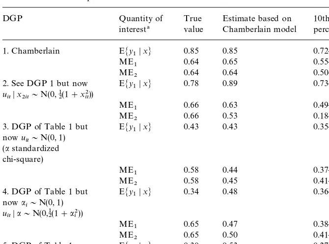
more interesting in practice, from a policy point of view. Such quantities can be estimated in a model which completely speci"es the conditional distribution of the individual e!ects and error terms, such as the Chamberlain (1984) model. This requires more assumptions than the semiparametric model and, therefore, can easily be misspeci"ed. If, in spite of misspeci"cation, the model leads to reasonable estimates of the quantities of interest, it will still be more useful for practical purposes than the semiparametric model. This makes it worthwhile to investigate how large the bias on the policy relevant parameters can be when a misspeci"ed Chamberlain model is used. We analyze this using the same Monte Carlo setup. We have computed the Chamberlain estimates for the same samples as before. Moreover, since the DGP used above di!ers from the Chamberlain model in various respects, we have also carried out the simulations for DGPs which are closer to the Chamberlain model. We focus on sample size
N"500.
The results are presented in Table 2. We consider the mean EMy1DxNand the marginal e!ects (keeping the "xed e!ect constant, cf. Chamberlain, 1984, pp. 1273}1274), ER/Rx
j1[EMy1Dx,aN]Dx(j"1, 2) atx"0 (the mean ofx). For"ve
di!erent DGPs, we present the three true values, the mean of the Chamberlain estimates for 500 Monte Carlo replications, and the 10th and 90th percentiles in these 500 replications. The "rst panel refers to the Chamberlain DGP (see Table 2 for details). In this case the Chamberlain model is not misspeci"ed, and the Chamberlain estimates perform quite well. Mean values and marginal e!ects are close to their true values, and the true values are always between the 10th and 90th percentile of the Chamberlain estimates. This shows that 500 observa-tions is enough to get reasonable"nite sample behaviour of the Chamberlain estimator, if the model is correctly speci"ed.
The second DGP di!ers from the "rst in the sense that the errors u
t are
heteroskedastic (u
tDxt&N(0,12(1#x22t)), as in speci"cation 6 of HonoreH). The
Table 2
Estimates for the mean EMy
1DxNand the marginal e!ects (MEj), based on the Chamberlain estimates in 500 Monte Carlo replications and for 5 di!erent DGPs
DGP Quantity of
!All quantities of interest are evaluated atx"0, the mean ofx. Marginal e!ects are computed as ME
j"EMR/Rxj1[EMy1Dx,aN DxNatx"0 (the mean ofx),j"1, 2.
three true values lie between the 10th and 90th percentile of the Chamberlain estimates. The estimate of the marginal e!ect of the second covariate}the one driving the heteroskedasticity}is very inaccurate, in accordance with the large variation in the estimates ofb2(not reported).
In the third DGP, we have used HonoreH 's speci"cation of "xed e!ects and covariates, as in Table 1. This implies that the conditional expectation of the
"xed e!ects is no longer linear in the covariates, and the distribution of the"xed
e!ects conditional upon the covariates is nonnormal, so that the Chamberlain model is misspeci"ed. In DGP 3, this is the only source of misspeci"cation}the error termsu
tare normal and homoskedastic. For this DGP, the Chamberlain
model is able to estimate the conditional mean of y
t quite well, but not the
marginal e!ects. These are underpredicted, and their true values exceed the 90th percentile of the distribution of the Chamberlain estimates. The source of this problem is that the estimates of P(y
t'0Dx) are too low (while there is only
a small bias onb).
In DGP 4, the marginal distribution of the"xed e!ects is standard normal, but the error terms are heteroskedastic in the same way as in the set up for Table 1. The marginal e!ects are underpredicted and they are similar to the previous case. However, the conditional mean of y
t is overestimated in
the Chamberlain model. Finally, DGP 5 is the same as in Table 1 and combines the various sources of misspeci"cation of the Chamberlain model. The Cham-berlain estimates have a high variance, re#ected in the large interval between 10th and 90th percentile of the parameter estimates, the conditional mean and the marginal e!ects. In particular, the estimate of the conditional mean is very inaccurate. Although the mean estimate deviates substantially from the true value, the true value is between the 10th and 90th percentile of the estimates. As in DGPs 3 and 4, the marginal e!ects are underestimated, and, for both covariates, their true value is near the 90th percentile of the 500 Chamberlain estimates.
These results imply that the conclusions on the marginal e!ects on the basis of the Chamberlain model can be biased if this model is misspeci"ed. The size of this problem varies with the type of misspeci"cation and may also be speci"c to our chosen Monte Carlo setup. In practical examples, misspeci"cation of the Chamberlain model may be much less of a problem than for our DGPs, and the advantages of the full speci"cation of the Chamberlain model could still out-weigh the drawback of misspeci"cation bias.
Alternatively, we could use the semiparametric model to give an approxima-tion of the marginal e!ects of interest. Under the additional assumption that
u
t and xt are independent, it is easy to show that EMR/Rxjt[EMytDx,aN]DxN"
b0P(a#b@
0xt#ut'0DxN. Since the distributions of a and u are not
speci-"ed, the probability in this expression cannot be computed, even if b0
were known. But it can be approximated by the sample fraction of positive values of y, or estimated nonparametrically at the given value of x. We will use the former in Section 7 to interpret the results of our empirical application.
5. Empirical application
vary over time or vary over time in a systematic way, the coe$cients in a"xed e!ects model should be interpreted as labor supply responses.3
We use data of the Dutch Socio-Economic Panel (SEP) of the years 1984}1988. Earnings are measured in each wave for all respondents. The natural logarithm of after tax earnings#1 is our dependent variable. The log transformation is used to capture the usual lognormal model as a special case, and to prevent a large impact of outliers. The #1 is added to account for the zeros, which has a negligible e!ect on the positive weekly earnings values.
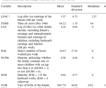
Our explanatory variables include the logarithm of weekly other family income (LOI; it includes the husband's earnings; again,#1 is added to account for zeros), the number of hours per week that the husband works (HM), and a dummy indicating whether the husband works (IEM). A dummy indicating whether the family contains children younger than six (DCH6) captures the e!ect of household composition; preliminary results indicated that other vari-ables related to children were not signi"cant. Also included are calender time (TIME), year of birth (YOB), and the woman's education level (EDF). Data on actual experience are not available.
Table 3 contains the variable de"nitions and sample statistics. In each of the
"ve waves, about 35% of the married females has a job. Comparing consecutive
years, 31% work in both years, 3% switch from not working to working and 3.5% switch from working to not working. Comparing waves which are two years apart, these percentages are 28%, 6%, and 6%. For three years di!erence, the percentages are 25.5%, 7.5%, and 8%, and for four years, they are 25%, 9%, and 10%, respectively. These"gures suggest that accounting for censoring is important.
In this section, we only use the 1987 and 1988 waves. We focus on the di!erences between the various estimates and on tests of the various speci" ca-tions. The economic interpretation will be addressed in Section 7. Our results are based upon 2278 women who are in both waves. We start with the Chamberlain (1984) model. The vector of regressors includes a constant term and the variables TIME, LOI, HM, DCH6, IEM, YOB, and EDF. To identify the model, the variables that are time-invariant or change linearly over time (YOB, EDF, TIME) are not included in the quasi-"xed e!ects. The estimated parameters for these variables can partly re#ect"xed e!ects.
3This raises the question why we do not estimate a model for hours worked instead of earnings. In some waves of the SEP, for those who do not change jobs, hours worked are not measured in each wave but taken from the previous wave. This makes hours worked infeasible for a panel data analysis. Moreover, hours worked are measured per week and show large spikes at 20 and 40 h (see Van Soest, 1995, for example). A censored regression model is not appropriate to deal with this.
Table 3
Variable de"nitions and sample statistics, 10,976 observations
Variable Description Mean Standard
deviation
Minimum Maximum
LINC! Log after tax earnings of the female (D#per week)
5.37 0.75 2.37 7.17
TIME Time (in years after 1900) 86.22 1.35 84 88 LOI Log of after tax other family
income, excluding female's earnings and unemployment bene"ts and earnings of children, including husband's
YOB Year of birth of the female 1947.79 10.96 1921 1969 EDF Education level of the female
(from 1: primary school only, to 5: university level)
2.31 0.97 1 5
!Based on 3837 positive observations only.
5.1. Chamberlain estimates
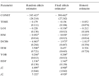
The estimates are presented in the third column of Table 4. For comparison, the results of the random e!ect model (with quasi-"xed e!ects independent of regressors) are presented in the second column. Some coe$cients in the
quasi-"xed e!ect are signi"cant, and the random e!ects speci"cation is rejected against
the"xed e!ect speci"cation by a Wald test. The parameter estimates for the time
varying regressors have the same sign but di!er in size: the random e!ects model overestimates the e!ect of children (DCH6) and employment of the husband (IEM).
The assumptions of normality and homoskedasticity were tested after the"rst round, using the tests of Chesher and Irish (1987). The form of heteroskedasticity that was tested for was VarMw
i#uitN"exp(j@xit). Both assumptions were
Table 4
Estimation results Chamberlain model and HonoreH estimates (¹"2) (standard errors in paren-theses)
IEM 3.500$ 0.457 0.526 0.429
(0.721) (0.663) (0.728) (0.076)
1related to DCH6 and in a2 related to DCH6 were
signi"cantly negative at the 1% level and the coe$cient ina
2related to IEM was signi"cantly
positive at the 5% level, indicating that it is important to allow for correlation between the individual e!ect and the regressors.
"No test on signi"cance carried out. #Signi"cant at the 5% level. $Signi"cant at the 1% level.
b0may be useful. The overidentifying restrictions are tested in the second step, by comparing the objective function value with the critical value of as27 distribu-tion. They are rejected at the 5% level (though this test is not valid if the"rst round estimators are inconsistent).
5.2. HonoreH estimates
The estimates following HonoreH (1992), based on (5) with A(x)"*x, are presented in the fourth column of Table 4. Sinceb0a!ectsoonly throughb@0*x, the coe$cients of YOB and EDF are not identi"ed. The estimates for HM,
DCH6 and IEM are similar to those in the Chamberlain model, with similar signi"cance levels. The time trend remains insigni"cant. The e!ect of other family income is negative, but its signi"cance level has dropped. The low signi"cance levels might be due to the fact that the HonoreH estimator is not e$cient.
To show the importance of taking account of the censoring, we present the OLS estimates on the"rst di!erences in the"fth column of Table 4. It is clear that these estimates are very di!erent from all others. For example, the OLS estimate of the parameter related to DCH6 is signi"cantly positive.
A speci"cation test for the "xed e!ects model (1) with the conditional ex-changeability assumption (A1), is a moment test based upon the smooth CMR for the truncated model, discarding observations with y
1"0 or y2"0 (see
Eq. (2.3) in HonoreH, 1992). Not conditioning onxleads to one UMR, which can be used to construct a method of moments test following Newey (1985). The test statistic is evaluated at the HonoreH (1992) estimate forb0. Under the null of no misspeci"cation, the test statistic is asymptotically chi-squared distributed with one degree of freedom. The null was rejected at the 5% level. An interpreta-tion of this result is that the data do not support the speci"c model assumptions (1) and (A1), although they may still support the weaker CMR assumption (4) used for estimation. Because of this, we only consider estimators based upon (4) and do not use more CMRs.
5.3. GMM with nearest neighbors
For applying e$cient GMM, observations withy
1"y2"0 are discarded in
nearest neighbors estimation, since they contribute zero too(y,b@ *x), whatever the value ofb. This reduces computing time substantially, reducing the dataset to 938 observations. YOB and EDF could, in principle, be included in the instruments, although their coe$cients inbare not identi"ed. Including them may change the weights in nearest neighbors estimation, but would also increase the dimension of the nonparametric regressions. Therefore, we do not include them.
Table 5
Nearest neighbors estimates (standard errors in parentheses)
Weights Uniform Triangular Quartic
Norm (benchmark model)
Invariant to linear transforms (5,50)! (0.057) (7,68)! (7,66)!
TIME 0.063 (0.104) 0.058 (0.058) 0.048 (0.058) LOI !0.237" (0.013) !0.214 (0.108) !0.203 (0.107) HM !0.031" (0.031) !0.031" (0.013) !0.030" (0.014) DCH6 !2.007# (0.342) !1.957# (0.349) !1.983# (0.344) IEM 0.505 (0.654) 0.580 (0.672) 0.503 (0.684) Invariant to multipliation (cf. Newey, 1993) (5,46)! (5,54)! (5,50)!
TIME !0.236HH (0.056) !0.040 (0.056) !0.059 (0.056) LOI !0.161 (0.118) !0.201 (0.110) !0.189 (0.115) HM !0.067# (0.014) !0.049# (0.013) !0.052# (0.014) DCH6 !1.871# (0.338) !1.835# (0.350) !1.850# (0.349) IEM 1.864# (0.660) 1.114 (0.657) 1.214 (0.662)
!(b,c):bnearest neighbors used in estimation ofD(x
1,x2) andcnearest neighbors used in estimation ofX(x1,x2). "Signi"cant at the 5% level.
#Signi"cant at the 1% level.
E.
Charlier
et
al.
/
Journal
of
Econometrics
95
(2000)
25
}
56
We investigated the sensitivity of the results for the numbers of nearest neighbors. Since the results with norm 1 are robust to the choice of weights, we focus on the model with norm 1 and uniform weights (the benchmark model). The results are presented in Table 6. Varying the number of nearest neighbors forDorXdoes not substantially change the estimates or their standard errors. The largest variation is found for the parameters of TIME and IEM, but these parameters always remain insigni"cant.
The standard errors in the benchmark model in Table 5 are smaller than their HonoreH counterparts in Table 4, though some of the di!erences are quite small. Signi"cance levels have increased, and the parameter of LOI is now signi"cant. The signi"cant parameters have the same sign and are of similar magnitude for both estimators. A Hausman-type test for misspeci"cation is performed, based upon comparing the two sets of estimates.4The null hypothesis of no misspeci" -cation was not rejected at the 5% level. This result was obtained for all speci"cations in Table 5.
5.4. GMM with series approximation
The results for GMM with series approximations are presented in Table 7 (see Appendix for computational details). Columns 2}4 contain the results for di!erent choices of the polynomials used in the series expansions. Standard errors are based on (14). They tend to be smallest in column 4, where most terms are used in the series approximation. The estimates of some parameters are rather sensitive to the choice of polynomials. HM and DCH6 are signi"cant and negative in all three cases. The results in the lefthand panel gave the lowest value for Newey's cross-validation criterion. As in the nearest neighbors case, the Hausman-type speci" ca-tion test does not reject the null of a correct speci"cation at the 5% level.
The major di!erence between series approximation and nearest neighbor results is that LOI is now insigni"cant. Estimated standard errors are not systematically lower or higher for either technique. The standard errors tend to be smaller than those of the HonoreH estimates in Table 4, but there are exceptions.
6. Extension to a panel with more than two waves
6.1. Balanced panel
In this section we extend our analysis to more than two waves. We will assume throughout that whether or not an individual is observed in a given
4This test requires a positive de"nite estimate for<MJN(bI!bK)N. We follow the standard approach: (10) implies thatJN(bI!bK)"CKv
N, withCKP1C,vNP$N(0,R) asNPR. Obtaining
Table 6
Sensitivity of the results for the number of nearest neighbors (uniform weights)$
Norm (3,50)! (7,50)! (5,45)! (5,55)!
Invariant to linear transform TIME 0.055 (0.057) 0.065 (0.057) 0.103 (0.057) 0.033 (0.058) LOI !0.263# (0.092) !0.226" (0.108) !0.244" (0.108) !0.196 (0.103) HM !0.030" (0.012) !0.029" (0.014) !0.031" (0.013) !0.029" (0.013) DCH6 !2.007# (0.334) !1.997# (0.337) !1.993# (0.351) !2.021# (0.340) IEM 0.785 (0.605) 0.482 (0.692) 0.502 (0.661) 0.396 (0.660)
!(b,c):bnearest neighbors used in estimation ofD(x
1,x2) andcnearest neighbors used in estimation ofX(x1,x2). "Signi"cant at the 5% level.
#Signi"cant at the 1% level.
$The cells contain parameter estimates and standard errors for the variables in the second column.
Table 7
E$cient GMM estimates based on optimal number of terms in the series approximation$
Base! IEM87,IEM88,IEM87*IEM88 HM87,IEM87,HM88,IEM88 HM87,DCH687,HM88,DCH688,HM87*HM87,H M87*DCH687,HM87*HM88,HM87*DCH688,D CH687*HM88,DCH687*DCH688,HM88*HM88, HM88*DCH688
TIME !0.048 (0.079) !0.047 (0.068) 0.060 (0.056) LOI !0.119 (0.099) !0.037 (0.095) !0.075 (0.072) HM !0.029" (0.012) !0.029# (0.011) !0.024" (0.012) DCH6 !1.836# (0.209) !1.919# (0.183) !2.897# (0.171) IEM 0.132 (0.807) 0.046 (0.789) !0.308 (0.757)
!A constant term was always included in the base.
"Signi"cant at the 5% level.
#Signi"cant at the 1% level.
$The cells contain the parameter estimates and standard errors based on (4).
E.
Charlier
et
al.
/
Journal
of
Econometrics
95
(2000)
25
}
56
wave is not related to the error termsu
t, i.e., we will not address the possibility of
attrition or selection bias. We"rst look at the balanced panel. The basic idea is to combine the conditional moment restrictions in (4) for each pair of panel waves. A su$cient assumption for this, together with regularity conditions similar to those for two waves, is the following generalization of HonoreH 's exchangeability condition:
(A2) For all s,t3M1,2,¹N, sOt, the distribution of (us,ut), conditional on
(a,x)"(a,x@1,2,x@
T)@, is absolutely continuous, and us and ut are
ex-changeable conditional on (a,x).5
This assumption is rather general and allows for many correlation structures between the random errors u
t. For example, it is less restrictive than the
assumption of complete exchangeability, that, conditional on (a,x), u"
(u
1,2,uT) has the same distribution as (up(1),2,up(T)) for any permutationn.
For example, the latter does not allow for"rst order autocorrelation in theu
t,
while (A2) does. Let*x
st"xs!xtand
o
st(b)"o(ys,yt,b@ *xst), (15)
whereois de"ned in (2). Then, for all 1)s(t)¹,
EMo
st(b0)DxN"0. (16)
These CMRs can be stacked into one vector de"ned as
o(b)"[o12(b),o13(b),2,o1T(b),o21(b),2,oT~1,T(b)]@. (17)
For anyA(x), this leads to the UMR
EMA(x)o(b0)N"0. (18)
The optimal choice forA(x) isB(x),D(x)@X(x)~1, where
D(x)"E
G
Ro(b0)Rb@
K
xH
,X(x)"EMo(b0)o(b0)@DxN. (19)Estimation of the optimal instruments requires a preliminary estimator forb0. HonoreH (1992) suggests to construct such an estimator on the basis of
A(x)"
C
*x12 0 0 . . 0 0 *x13 0 . . 0
. . . .
0 . . . . *x
T~1,T
D
. (20)
5For some of our estimators, it is su$cient to impose the slightly weaker condition of exchangea-bility conditional upona,x
This is the estimator which minimizes the equally weighted sum of the criterion functions of the HonoreH (1992) estimates for all pairs of waves. Combining (18) and (20), more moments than parameters are used in estimation, so, for example, GMM with the optimal weighting matrix can be used. This requires estimating the optimal weighting matrix. For this, a consistent preliminary estimator for
b0 can be constructed giving equal weights to the moments *x
stost. This is
convenient since the estimator can be obtained by minimizing a strictly convex objective function. Given these preliminary estimates, the optimal weighting matrix can be estimated and one Newton}Raphson step towards the solution of the optimal GMM estimator based on (18) and (20) can be performed. We refer to this estimator, which is asymptotically equivalent to GMM with the optimal weighting matrix, as the HonoreH estimator. The many moments used in estima-tion can be used to test for overidentifying restricestima-tions.
The HonoreH estimator for b0 can be used as a starting point to perform e$cient GMM with the optimal choice forA(x), i.e.B(x). As in Section 3, we will use the asymptotically equivalent estimator which goes one Newton}Raphson step towards the solution of the e$cient GMM minimization problem. We refer to this estimator as (e$cient) GMM. Its drawback is the large dimension of the nonparametric estimation ofB(x) if the dimension ofx
tor the number of time
periods is not very small, as is the case in our empirical example. Alternatively, we can use that EMo
st(b0)Dxs,xtN"0 for each 1)s(t)¹
and use the two step GMM estimator for¹"2 introduced in Section 3 for each combination (s,t), 1)s(t)¹. To restrict the estimates forb0to be the same for each combination (s,t), the"nal step in estimation is then Asymptotic Least Squares (ALS) (see, for example, Kodde et al., 1990). This procedure, which we will refer to as the ALS estimator, might asymptotically be less e$cient than two step e$cient GMM, but is easier from a practical point of view. Moreover, it can also be applied to unbalanced panels.
Using the balanced subpanel with complete information for all"ve waves and with at least one nonzero observation ony
tleads to only 243 observations which
is too few for our high dimensional nonparametric regression. Therefore, we applied the estimators to the balanced subpanel for the years 1986}1988 (¹"3). The dataset (withy
it'0 for at least onet) consists of 823 individuals. We use
norm 1 and nearest neighbors with uniform weights. Cross-validation was used to determine the optimal numbers of nearest neighbors forDandX(for ALS, to limit the computational burden, the optimal numbers are computed for 1987 and 1988 and used for all pairs of waves).
The HonoreH estimates are presented in the second column of Table 8. Only the dummy for young children (DCH6) is signi"cant. The results for the other two estimators using all covariates but TIME to compute the distances needed for nearest neighbors, are presented in Columns 3 and 4. Although their signs are the same, the magnitudes and standard errors for the ALS and GMM estimates are rather di!erent. The GMM estimates are all signi"cant but one.
Table 8
Estimation results with more than two waves (standard errors in parentheses)
Parameter HonoreH estimator
E$cient GMM, fully!
Two stage ALS, fully!
E$cient GMM, partly"
Two stage ALS, partly"
HonoreH estimator
Two stage ALS, fully!
Panel Balanced, Balanced, Balanced, Balanced, Balanced, Unbalanced, Ubbalanced, '86}'88 '86}'88 '86}'88 '86}'88 '86}'88 '84}'88 '84}'88 TIME 0.058 0.047% 0.049 0.026% 0.085 !0.002 0.008
(0.043) (0.001) (0.048) (0.002) (0.050) (0.029) (0.028) LOI !0.093 !0.066% !0.007 !0.073% !0.561 !0.068 !0.153$
(0.082) (0.010) (0.064) (0.008) (0.422) (0.052) (0.065) HM !0.004 0.001% !0.006 !0.006% 0.001 !0.012 !0.012
(0.008) (0.0004) (0.009) (0.0004) (0.011) (0.006) (0.006) DCH6 !2.357$ !1.353% !2.297% !1.623% !2.405% !2.680% !2.484%
(0.254) (0.163) (0.265) (0.157) (0.266) (0.178) (0.184) IEM 0.193 0.006 0.262 0.345$ 0.855 0.416 0.361
(0.557) (0.029) (0.540) (0.030) (0.967) (0.292) (0.356)
NN# (6,95) (8,65) (6,135) (14,120) (5,50)
Objective function 21.65 16.15 18.70 69.11 58.66
!Fully: the moments conditional on (LOI,HM,DCH6,IEM) are used in estimation.
"Partly: only the moments conditional on (HM,DCH6) are used in estimation.
#(a,b): number of nearest neighbors used estimatingDandX, respectively.
$Signi"cant at the 5% level.
%Signi"cant at the 1% level.
E.
Charlier
et
al.
/
Journal
of
Econometrics
95
(2000)
25
}
However, for ALS only DCH6 is signi"cant. Compared to the results based on 1987}1988 (Tables 5 and 6), the e!ect of the husband's hours worked (HM) has disappeared.
We have only 823 observations, but the GMM estimates use a twelve-dimensional nonparametric regression. To avoid this problem of twelve- dimensional-ity, we also present (in Columns 5 and 6 of Table 8) estimates based on conditioning only on all periods' values for HM and DCH6, the two most important explanatory variables according to Section 5. This reduces the dimen-sion of the nonparametric regresdimen-sion from 12 to 6. It leads to some substantial changes in the parameter estimates for GMM. All ALS estimates but one remain insigni"cant. The signi"cant negative sign of DCH6 remains.
The objective function value (bottom row of Table 8) can be used to perform a test on overidentifying restrictions in the HonoreH estimates and the two-stage ALS estimates. The hypothesis of no misspeci"cation could not be rejected at the 5% level for the two-stage ALS estimates in Column 4. For the HonoreH
estimates and the two-stage ALS estimates in Column 6, this hypothesis is rejected at the 5% level, but not at the 1% level. We also performed a Hausman test based upon the di!erence between GMM estimates and HonoreH estimates. The null of no misspeci"cation was rejected at the 1% level.
6.2. Unbalanced panel
Letc
st"1 if (ys,yt,xs,xt) is fully observed and zero otherwise. We assume that
the distributions of c
st and ys,yt are conditionally independent for given
x"(x@1,2,x@T)@(no selection or attrition bias). We then have
EMc
stost(b0)Dx1,2,xTN"0, for alls,t, with 1)s(t)¹. (21)
Since we do not observex
1,2,xTfor all individuals, we use the weaker CMR
EMc
stost(b0)Dxs,xtN"0, for alls,t, with 1)s(t)¹. (22)
We apply the two waves estimation procedure for each (s,t) separately and use ALS to estimate b0. To limit the computational burden we determine the smoothing parameters for (s,t)"(1, 2) and use the outcome for all pairs of waves.
The unbalanced panel (for 1984}1988) consists of those individuals who are observed in at least two waves, with positive earnings at least once. This leads to a sample of 1351 individuals. We use uniform weights and norm 1 and all elements in (x
s,xt) except for TIME are included in the distance calculations
needed for nearest neighbors. The optimal numbers of nearest neighbors are the same as in Section 5.
The HonoreH estimates are presented in Column 7 of Table 8. Again, DCH6 is the only signi"cant variable. Compared to the balanced sub-panel 1986}1988,
standard errors have decreased. The ALS estimates (Column 8) are similar to the HonoreH estimates, the main di!erence is that other income (LOI) is also signi"cant at the 5% level. Most ALS standard errors are larger than the HonoreH standard errors, in contrast to what asymptotic theory predicts. At the 5% level, the test on overidentifying restrictions results in rejecting the hypothesis of a correct speci"cation for the HonoreH estimate (69.11's245_0.05"
60.61) but not for two stage ALS (58.67(s2 45_0.05).
7. Economic interpretation
Our model explains earnings of married females, which are determined by hours worked and hourly wages. The Chamberlain (1984) estimates in Table 4 already suggest that"xed e!ects are important, since the random e!ects model is rejected against the quasi-"xed e!ects alternative. Fixed e!ects in the labor supply decision have a clear interpretation in a life cycle context. The hourly wage is mainly determined by human capital variables that hardly vary indepen-dently over time, so that"xed e!ects and human capital e!ects on hourly wages cannot be disentangled.
In the"xed e!ect models, only the variables of the time varying regressors are identi"ed. These mainly refer to the labor supply decision. From the results we conclude that, ceteris paribus, the presence of a child less than 6 yr old has a strong negative e!ect on the woman's labor supply. The magnitude of the e!ect is much smaller in the"xed e!ects model than in the random e!ects model. Based upon the approximation discussed at the end of Section 4, the e!ect of a young child would be a reduction of average log earnings of about !1.7 (parameter estimate!4.86, times employment rate 0.35) in the random e!ects model. In all "xed e!ects models it would be about !0.7. This is the most robust "nding in the paper. The negative e!ect is in line with the common
"nding in the female labor supply literature.
According to most of the estimates, other family income (mainly husband's earnings) has a negative e!ect, which is often signi"cant. According to the results in Column 8 of Table 8, the (geometric) average of women's earnings (#1) would fall by about 0.05% if their husbands'net income would increase by 1%. In a standard life cycle model without uncertainty, the elasticity would be zero, because family consumption would be smoothed for changes in family income. Our results suggest that changes in other family income may partly be unan-ticipated, and will lead to an adjustment of the family's permanent income.
We"nd some evidence suggesting that, ceteris paribus, the number of hours
the husband's participation, we also included a dummy for the husband's employment, but this was never signi"cant.
We"nd that the joint impact of time and year of birth (or age) is insigni"cant.
Our "xed e!ects model does not allow to distinguish between the (probably
positive) time trend and the (probably negative) age e!ect. We also estimated the model with additional explanatory variables, such as the number of children in the family younger than 18, and age squared. In none of the estimation results these variables were signi"cant. Including them had little e!ect on the other estimates.
Our main"ndings are interpreted in terms of women's labor supply behavior. This raises the question whether an equation for hours of work instead of earnings would lead to di!erent results. We have already explained above why our data are better equipped for analyzing earnings rather than hours worked. Still, we have estimated the same type of model for hours worked. This led to the same economic conclusions as those given above.
Finally, it should be noted that for¹"2 most speci"cation tests led to the conclusion that the censored regression"xed e!ects model cannot be rejected. This is somewhat surprising, since in cross-section settings, the censored regres-sion model is often found to be inferior to a less restrictive sample selection model (see, for example, Melenberg and Van Soest, 1996). Apparently, "xed e!ects may make a large di!erence here. On the other hand, tests including more time periods often led to the conclusion that the censored regression"xed e!ects model should be rejected.
8. Conclusions
We have considered estimators for the censored regression model, compared them in a Monte Carlo experiment, and applied them to panel data on earnings of married females. We have focused on the semiparametric estimator for models
with"xed e!ects designed by HonoreH (1992), and e$cient GMM estimators based
upon this estimator, following Newey (1993). For two panel waves, Monte Carlo results suggest that the GMM technique works well in practice, though many observations are needed before e$ciency gains compared to the HonoreH estimator are obtained. We have also compared the semiparametric estimators with the parametric Chamberlain (1984) estimator, which models the"xed e!ect in terms of a linear combination of covariates and an error term, and assumes normality and homoskedasticity. Such an estimator has the advantage that the model is fully speci"ed such that the model can be used to compute e!ects other than the slope coe$cients, such as marginal e!ects of covariates on the observed dependent variable. Monte Carlo results, however, suggest that estimates of such e!ects can be biased if the Chamberlain model is misspeci"ed.
For more than two panel waves, we have compared the estimator proposed by HonoreH (1992), an e$cient GMM estimator for a balanced panel, and
Asymptotic Least Squares estimators using either the balanced subpanel or the complete unbalanced panel.
Our empirical results show that taking account of"xed e!ects substantially changes the conclusions on the sensitivity of female labor supply for the presence of children, other family income, the husband's hours of work, etc.
The semiparametric estimators are fairly easy to compute, though the e$cient GMM estimator requires the choice of smoothing parameters. Our sensitivity analysis for a panel with two waves shows that the results are not very sensitive to the choice of these parameters. Still, our results are somewhat mixed. Where the e$cient GMM estimators should asymptotically be more e$cient than HonoreH 's estimator, they do not always lead to unambiguously smaller esti-mated standard errors.
The e$ciency gains are obtained by an optimal construction of unconditional moment restrictions, given the choice of a conditional moment restriction. An alternative would be to consider more conditional moment restrictions. HonoreH
(1992) notes that there is an in"nite number of conditional moments one could consider. In our Monte Carlo experiment, using a second conditional moment only leads to a small e$ciency gain. In our empirical example Hausman speci" ca-tion tests suggest that the condica-tional moment restricca-tion used by HonoreH is valid but that the assumption of conditional exchangeability might not hold.
In principle, the GMM framework used here could also be extended to selection models. Kyriazidou (1997) introduces a consistent estimator allowing for a general structure of"xed e!ects. More e$cient estimators using this estimator as a starting point, could be obtained along the same lines as described in this paper.
Acknowledgements
We thank Bo HonoreH, Marno Verbeek, Myoung-Jae Lee, Gerard Pfann, an associate editor and two referees for helpful comments. Research of the third author is possible due to a fellowship of the Netherlands Royal Academy of Arts and Sciences (KNAW). We are grateful to Statistics Netherlands (CBS) for providing the data.
Appendix A
We brie#y discuss the assumptions needed for Theorems 1 and 2, drawn from Newey (1993), for our empirical application, and present some computational details for applying Theorem 2.
A.1. Assumptions for Theorem 1
continuous on the interior of a compact set, continuously di!erentiable on a tiability we need that 1(!y
2(b@ *x(y1) is continuous in b in E with
probability one. In our application,y
1andy2are the log(female's earnings#1),
and thus mixed discrete-continuous (zero or positive); x contains LOI, the log(other income#1), and HM, hours worked by the husband, which are also mixed discrete-continuous. However, notice that female's income and other income or hours worked by the husband generally will not simultaneously be equal to zero, so that the set at which 1(!y2(b@ *x(y1) is discontinuous will be negligible. Alternatively, one could modify Newey's approach by basing it upon Pakes and Pollard (1989), similar to HonoreH (1992), in which case one will need as requirement continuity of P(!y
2(b@ *x(y1Dx). Assumption 4.2 of Newey (1993) is not required,
because we do not apply GMM, but the two step procedure. Newey (1993)'s Assumption 4.3 deals with properties of the "rst round estimator,
bKH in our case, which can be checked partly. The crucial identi"cation part of this assumption is that EM*xo(y
1,y2,b@ *x)N"0 is uniquely satis"ed
at b0. This is proven in HonoreH (1992). The condition that the "rst stage estimator should be based on a GMM type of objective function is not satis"ed here, but Lemma A.1 of Newey (1993) can be easily adapted such that Theorem 1 still goes through for the"rst stage estimator used here. Assumption 4.4 of Newey (1993) requires uniform boundedness in¸2norm of
DDo(z,b)DD4, DDRo(z,b)/RbDD4, and ER2o/Rb Lb@E, and a Lipschitz condition on ER2o/RbRb@E (all on a neighborhood E of b
0). From (2), it follows that this
condition will be satis"ed if eighth order moments ofzexist. Thus the required assumptions are stronger than those required by HonoreH (1992). Assumption 4.5 of Newey (1993) is not needed because D is estimated nonparametrically. The only additional assumption in Theorem 1 of Newey (1993) concerns the rate at which the number of nearest neighbors used in estimation tends to in"nity asN tends to in"nity.
A.2. Additional assumptions for Theorem 2
Apart from some regularity conditions, Assumption 5.1 of Newey (1993) contains an assumption on the existence of EMDDD(x,g)DD2a@(a~2)`dN"
EMDD*xDD2a@(a~2)`dNfor somea'2,d'0. The condition onQandQK in Assump-tion 5.1, is satis"ed because we chooseQ"QK"I.
Assumptions 5.3 and 5.5 are veri"ed for our speci"c application. We aim at approximatingB(x)"!*x F(x), with the real valued functionF(x) given by (23) below. The function F(x) is approximated using a polynomial base in elements of x. More formally, let a
K(x)"[a1K(x),2,aKK(x)]@ represent the
elements of the polynomial base. We then approximateF(x) by c(@a
K(x), where
c( still has to be determined (see below). Checking that Newey's assumptions 5.3 and 5.5 (that imply his Assumptions 5.2 and 5.4) are satis"ed is easy here: Choosea
kK(x)"pk(x) [withqj(xj)"xj].xshould contain at least one
continu-ously distributed component with density assumed to be bounded away from zero on (0,R). From a practical viewpoint, we can let LOI do the job. We tried estimation both with LOI included and excluded. The reported results are without LOI. Excluding LOI only changed the parameter estimates related to LOI and IEM. The elements in*xare not linearly dependent, implying that the smallest eigenvalue ofM*x*x@NX(x) is bounded away from zero. By choosing the degree of the approximating polynomial increasing inK,J(K)"Kand¸
K"I,
Assumption 5.3 is satis"ed except for the boundedness of theqj. The latter is not a problem because boundedness can be relaxed without a!ecting the results (Newey, 1993, p. 440). Assumption 5.5 of Newey (1993) is also easy to check, since Ris only one dimensional here. With a
kK(x)"pk(x) and J"K, we can
choosec
j"c1j,j"1,..,K, so that Assumption 5.5 is satis"ed.
A.3. Computation of series approximations
In the series approximation of the optimal instruments we follow the proced-ure described in Newey (1993, pp. 435}438). Here, we discuss the series approxi-mation in more detail. In the censored regression panel data model we can write
B(x)"!*x F(x), with
F(x)"EM1(!y2(b@
0*x(y1)DxN[EM[o(y1,y2,b@0*x)]2DxN]~1. (23)
In this case, instead of having to approximate a vector of functions ofx, we only have to approximate the real valued function F(x). This function is approxi-mated by a series expansionR
kckakK(x), as discussed above. For the functions
a
kK(x) we use polynomials in elements ofx. For the moment, assume that the
number of terms in the series approximation (i.e.,K) is given. We now need to estimatec"(c1,2,cK)@. Newey (1993, p. 436) gives an infeasible estimatorc6that
minimizes the mean-square distance between the function B(x) and the series approximation!*x[Rkc
kakK(x)]. In this distance function, a positive de"nite
matrixQappears. For simplicity and because no good guidelines for choosing
Q are available, we choose Q equal to the identity matrix. The resulting estimatorc6is infeasible because it depends on, among other things,B(x), which is not observed. Therefore, the estimator c6 is rewritten in such a way that constructing a feasible estimator is easy. The resulting estimatorc6is presented in Newey (1993, Eq. (5.3)), and c(, the feasible equivalent of this estimator, is obtained by replacing the expectations by sample averages andb0bybKH. Then
c( is used to approximate the optimal instrumentsB(x) by !*x[R
kc(kakK(x)],