A model for light competition between vegetable crops and
weeds
M. Ro¨hrig *, H. Stu¨tzel
Institute for Vegetable and Fruit Crops,Uni6ersity of Hano6er,Herrenha¨user Strasse2,D-30419Hanno6er,Germany
Received 27 July 1999; received in revised form 13 March 2000; accepted 15 May 2000
Abstract
A precise prediction of the yield losses inflicted by weeds is the basis of decisions in weed management. Hitherto, only rough estimates, which neglect the specific production situation, have been available for vegetable crops. In this study a simple simulation model was developed to estimate yield loss by radiation competition as a function of environmental variables. In the model, the distribution of incoming photosynthetically active radiation (PAR) in the canopy is calculated using a spatially highly resolved approach. Growth is calculated as a function of absorbed radiation and its utilisation. Newly produced dry matter is allocated to roots and shoots, the latter comprising vegetative and reproductive organs according to the developmental stage. Vegetative shoot dry matter is partitioned according to the main functions of radiation interception (leaves) and structural stability (stems and petioles). The resulting leaf area is distributed in the canopy according to the spatial expansion of individual plants. Calibration runs revealed uncertainties predicting the growth ofChenopodium albumand a high sensitivity of crop yield to leaf area development of the weed. Using the area of green leaves (LAI) ofC.albumas input gave a close correspondence between simulated and observed crop yield loss. Since plant height ofC.albumis calculated as a function of leaf area, this variable has a multiple effect on radiation absorption. A first evaluation with an independent data set likewise gave an acceptable prediction. To reduce model complexity, a simplified version is proposed. © 2001 Elsevier Science B.V. All rights reserved.
Keywords:Simulation model; Weed competition; Cauliflower;Chenopodium album
www.elsevier.com/locate/eja
1. Introduction
To optimise weed control measures, reliable estimates of the expected impact on crop yield are
required. Hence in vegetable production, ‘critical periods’ of weed competition were defined as the time interval during which a crop has to be kept weed free to achieve maximum yield (Nieto et al., 1968; Roberts, 1976). ‘Critical periods’ were deter-mined empirically for a range of crops (Hewson and Roberts, 1973; Weaver, 1984; Qasem, 1992), but this concept ignores the influence of the site-specific ecological and agronomic conditions and * Corresponding author. Present address: Danish Institute
of Agricultural Sciences, Department of Agricultural Systems, Research Centre Foulum, P.O. Box 50, DK-8830 Tjele, Den-mark. Tel.: +45-89991780; fax:+45-89991200.
E-mail address:[email protected] (M. Ro¨hrig).
is therefore not an adequate method for decision support in weed control. Consequently, the effects of weeds on crop growth and yield can only be accurately quantified, if the competitive system is simulated as authentically as possible considering the specific production situation.
A large number of simulation models were de-veloped to extrapolate the results of experimental field studies. These are in general empirical regres-sion models describing yield losses statistically by an equation based on one or more parameters such as weed density, relative leaf area or relative time of weed emergence (Cousens et al., 1987; Kropff and Spitters, 1991; Lotz et al., 1992). Since the estimated parameter values often vary consid-erably between locations and years, their potential for extrapolation is limited. To achieve more uni-versally valid results, resource-consuming field ex-periments would have to be carried out repeatedly for additional calibrations. Furthermore, the co-efficients of empirical models commonly lack a physiological basis thus giving no insight into the causal relationships underlying crop – weed com-petition. Competition in the sense of process-ori-ented models is defined as the distribution of growth-limiting factors between species in a vege-tation canopy and the efficiency of each species to use these resources for biomass production (Spit-ters, 1990). These resources comprise radiation, nutrients and water, which are modelled with a varying degree of detail dependent on the situa-tion to be examined. With this approach, crucial determinants of crop – weed competition can be identified and used to manipulate the competitive relationships. Moreover, processes not well under-stood are disclosed thus suggesting fields for fur-ther investigations. Most mechanistic models on competition between crops and weeds (Spitters and Aerts, 1983; Wilkerson et al., 1990; Kropff and Spitters, 1992; Debaeke et al., 1997) were derived from models of crop growth in monocul-ture (van Keulen et al., 1982; Wilkerson et al., 1983; Spitters et al., 1989; Williams et al., 1989). To quantify the radiation interception of compet-ing species, the canopy is divided into horizontal layers in which the species have a different share of total leaf area. In principle either the height (Spitters and Aerts, 1983; Spitters, 1989) or the
number of layers (Wilkerson et al., 1990) is held constant. This approach is basically one-dimen-sional assuming a homogeneous leaf area distribu-tion within a layer. To account for a horizontally heterogeneous leaf area distribution in row canopies, Wilkerson et al. (1990) proposed an empirical approach by calculating radiation inter-ception based on a competitive factor and an ‘area of influence’. The latter is defined as ‘a rectangle of width equal to the rowspacing and length down to the crop row equal to the weed canopy diameter’. After validation, these models can be applied to systems in other environments (Kropff et al., 1993) but are rarely used in practi-cal weed management because of the large num-ber of parameters.
In the simulation study presented here, special attention is drawn to the competition for radia-tion in heterogeneous plant canopies. This consid-ers the particular situation of vegetable production where (a) field crops are usually planted in widely spaced rectangular patterns thus being single plants rather than ‘closed’ or row canopies and (b) the competitive situation is mainly reduced to radiation competition due to the common practice of amply irrigating and fer-tilising. In this situation, the spatial development of competing plants and their morphological adaptation to unfavourable growth conditions strongly influences the distribution of radiation within the canopy. Therefore, a three-dimensional radiation interception model (Ro¨hrig et al., 1999) was extended to calculate the radiation intercep-tion in multispecies canopies. This improves exist-ing approaches because the horizontal heterogeneity of leaf area distribution and its affect on competition can be described explicitly. The model was used to analyse the competition between Chenopodium album L. and cauliflower (Brassica oleracea L. convar. botrytis var. botry
re-duce complexity and to adapt the simulation to an intended use in decision support.
2. Materials and methods
2.1. Experiments
The effects of interspecific radiation competi-tion between common lambsquarters (aka. fat hen, Chenopodium album L., Conrad Appel, Darmstadt, Germany) and cauliflower (Brassica oleracea L. convar. botrytis var. botrytis L. cv. Fremont, Royal Sluis, Neustadt, Germany) were examined in field trials in 1994 and 1995. The trial in the second year was carried out as a spring (‘experiment 1’) and a summer planting (‘experi-ment 2’) with identical layouts (Table 1). The experiments were made on a silty loam at the
experimental station in Ruthe near Hanover, Ger-many. To achieve different degrees of competi-tion, planting density of C. album was varied at two levels. In addition to mixed stands, plots with
C. album in monoculture were planted on both densities. The experiments were set up in com-pletely randomised blocks with four replications. Within each plot, separate subplots were used for four successive samplings throughout the growing period.
2.1.1. Culti6ation
Cauliflower seedlings were cultivated in a green-house until the transplants had an average fresh weight of c. 5 g and had four to five leaves. At least 1 week prior to planting the transplants were hardened off in a cold frame. In the field, the plants were arranged in a rectangular pattern in 1994 and in an isometric pattern in 1995.
Nitro-Table 1
Cultivation and sampling data of field experiments Cauliflower
1994 1995 experiment 1 1995 experiment 2
18 February
Sowing date 24 February 8 June
18 April 24 April 18 July
Date of transplanting
Harvest dates 16 May 24 May 9 August
31 May 9 June 23 August
13 September 28 June
20 June
10 July 9 October
1 Julya
Planting pattern (m) 0.5×0.6 0.45×0.52 0.45×0.52 3.33
Plants (m−2) 4.27 4.27
Plot area (m2) 8.4×4.0 7.28×2.0 7.28×2.0
Plants per harvest 10 4 4
Chenopodium album
Sowing date 19 April 3 April 27 June
20 July –
Date of 3 May
transplanting Plants (m−2)
Target: 25, emerged: 24
Low density Mixed: 12.8, pure: 17.1 Mixed: 12.8, pure: 17.1 Target: 50, emerged: 41
High density Mixed: 38.5, pure: 42.7 Mixed: 38.5, pure: 42.7 Five or three (early or late
gen fertilisation was given shortly before and 4 weeks after transplanting: after soil sampling, the mineral N supply was replenished to 130 kg N ha−1 at the first and to 270 kg N ha−1 at the
second application (Lorenz et al., 1989). In 1994,
C.albumwas sown by hand directly into the field. After a germination test, a quantity of seeds ap-propriate to obtain target densities was mixed with quartz sand and spread out uniformly over the plot. In low density plots, the target density was achieved, but it fell short in high density plots (Table 1). Still, a considerable variation between the treatments could be expected. Due to a long juvenile phase, the onset of competition with cauliflower was notably delayed. To achieve early competition, C. album plants were raised and transplanted to the field for the 1995 experiments. Four to five seeds were laid into peat-filled cone-trays and singled after emergence. After raising the seedlings in a greenhouse, they were trans-planted when having about three nodes and an average height of 3 cm. The weed densities were achieved by placing one or three C. album be-tween two cauliflower plants for low and high density plots, respectively. In pure weed stands, the same pattern was used, except that the posi-tion of the cauliflower plant was filled by another weed. This resulted in slightly higher planting densities in pure than in mixed stands. All plots were well irrigated to avoid water limitations and weeds emerging spontaneously were removed by hand. Pests and insects were controlled chemically for both crops and weeds.
2.1.2. Data collection
At four successive sampling dates, a number of cauliflower andC. album plants were taken from the designated sub-plots. Plants were dug out to a depth of c. 20 cm; the roots were washed and separated from the shoot just above the first lateral root branching off. Measurements of shoot length from base to top and its greatest width gave the plant height and diameter, respectively, both with an accuracy of c. 5 mm. The shoots were divided into stems (including petioles), green leaves, senescent leaves and reproductive organs (only cauliflower). All plant parts were dried for at least 3 days at 100°C and weighted. The area of
green leaves was measured with a LI-COR 3100 Area Meter (LI-COR Inc., Lincoln, NE, USA). From these data the green leaf area index (LAI) was calculated. Hourly data of air temperature, global incoming radiation and relative humidity were supplied by an on-site automatic weather station (Campbell Scientific, UK).
For further details see Ro¨hrig et al. (1999) and Ro¨hrig (1999).
2.2. Model description
The model presented here was derived from a crop growth simulation for faba beans (Stu¨tzel, 1995a,b), which calculates plant growth based on the insolation. The profile of absorbed radiation in the canopy is computed assuming a leaf area distribution in three dimensions. From the ab-sorbed radiation and the efficiency of its use, the total growth rate of the competing species is estimated. The biomass produced is partitioned into the various plant organs. From the leaf dry weight and the specific leaf area, the LAI is calculated, which is distributed in the canopy according to plant positions and dimensions. De-velopmental processes such as vernalisation and ontogeny are modelled as a function of ambient temperature (Kage and Stu¨tzel, 1999).
2.2.1. Calculations
Fifty percent of the incoming global radiation (400 – 3000 nm) is assumed photosynthetically ac-tive radiation (PAR, 400 – 700 nm). The thermal time scale is defined in the model as the tempera-ture sum TS (°C day):
TS=%TavwithTav=
Tmin+Tmax
2 (1)
where Tav, Tmin and Tmax are the daily average,
minimum and maximum temperatures in °C, re-spectively. A base temperature of 0°C for both cauliflower (Wurr et al., 1990; Grevesen and Olesen, 1994) and C. album (Angus et al., 1981) was used.
2.2.2. Growth processes
complete canopy volume is divided into cubic subunits, which are either empty or filled with leaf area. Leaf area of each plant of a species is distributed in a geometric foliage envelope, which is defined in the model domain by plant height, diameter and position. Foliage envelopes may overlap resulting in a multiple occupation of a cube by one or more species. Radiation transmis-sion is then calculated by following the path of a solar ray through the canopy volume until ground level is reached. The absorption of diffuse radia-tion is calculated by selecradia-tion and integraradia-tion of solar rays from 15 directions according to the Gaussian integration algorithm (Goudriaan, 1986). This routine is also used to integrate the diurnal course, yielding a daily total of absorbed radiation,Ia (MJ m
−2, Eq. (19) in Ro¨hrig et al.,
1999), for each species. The increase of total plant biomass,WT (g m−2), is calculated as a function
of Ia and the radiation-use efficiency, RUE (g
MJ−1):
dWT
dt =IaRUE (2)
In 1995 it was found that (a) RUE of cauliflower showed a seasonal variation between the experi-ments and (b) crop dry matter decreased due to profound shading byC.album. The seasonal vari-ation of RUE can be attributed to a differing insolation that was also found in potatoes (Man-rique et al., 1991). A log – normal function was used to describe both findings:
RUE=e1+e2e
−0.5(ln(I0, c/e3)/e4)2
(3)
where e1 to e4 are calibration constants and I0, c
(MJ m−2) is the daily radiation incident on a
horizontal plane above the cauliflower plants. The constante1is the minimum of the function ande3
denotes the maximum, i.e. the irradiance at which RUE is maximum. If I0 (MJ m−
2
) is the insola-tion and Ia,t (MJ m
−2
) denotes the radiation absorbed by the entire canopy, then the irradiance above species S, I0,S, amounts to:
I0,S=I0−(Ia, t−Ia,HS) (4)
where Ia,HS (MJ m
−2) is the radiation absorbed
by the canopy from the height of species S, HS,
down to ground level. In the case of monospecific
stands I0,S equals I0; in mixtures the term in
parentheses represents the radiation absorbed by species with leaf area between the top of the canopy and the top of the species under consider-ation. Newly produced biomass is allocated to root, WR (g m−2), and shoot dry matter, WSh (g
m−2), using an allometric growth equation
(Per-sall, 1927). As shown by Kage and Stu¨tzel (1999), Eq. (18), the growth rates of plant organs growing allometrically are obtained by:
dWSh
Considering roots and shoots, the term ea is the
ratio between the initial weights (Persall, 1927) and the allometric growth coefficient b denotes the fixed ratio between the relative growth rates (Thornley and Johnson, 1990).
For cauliflower, the shoot dry matter is allo-cated to vegetative,WV(g m
−2), and reproductive
organs,WG(g m
−2), but only after curd initiation
(Kage and Stu¨tzel, 1999). They proposed that during the reproductive phase the ratio of curd growth rate to shoot growth rate increases logisti-cally in time. On the transition from the exponen-tial to the linear phase of the logistic function, the sink strength of the curd becomes substantial. At this point, it is assumed that a fraction of the vegetative shoot dry weight is reallocated to the curd. The reproductive growth rate is then:
dWG
where f is a logistic growth function of thermal time after curd initiation (see Eq. (21) in Kage and Stu¨tzel, 1999) and rt (°C−1
day−1
) is the translocation rate. For the distribution of vegeta-tive shoot dry matter into stems,WS(g m
−2), and
leaves,WL(g m
−2), the approach of Stu¨tzel et al.
dWL
where h and g are constants. In case of low irradiance Eq. (3) may become negative. Since stems and roots are less physiologically active, these losses are solely attributed to leaf dry weight and all other growth rates are set to zero. It is furthermore assumed that the leaf area in-dex, L (m2 m−2), is directly linked to leaf dry
newly formed leaves. Eq. (8) also implies that per unit dry weight loss, leaf area is decreasing only by half the actual leaf area ratio. SLA is a con-stant input parameter for C. album, but in cauliflower it is made a function of the radiation environment quantified by Alt (1999) (personal communication):
SLA=0.059I−0, c, av0.85 (9)
where I0, c, av is I0, c (MJ m−2) as a running
aver-age of 5 days. This relationship takes into ac-count leaves becoming thinner when growing under low radiation. Dry matter production and distribution ofC. album are quantified in Ro¨hrig (1999). The radiation-use efficiency and the co-efficients of the allometric growth equation are estimated and the effects of competitive stress on the growth processes are discussed. All data from the 1995 experiments were used for calibration.
2.2.3. De6elopmental processes
Vernalisation and flower initiation in cauliflower are modelled by the temperature sum approach of Wiebe (1979) as modified by Kage and Stu¨tzel (1999). The spatial expansion of cauliflower plants is calculated as a hyperbolic function of stem dry weight for plant height, H
(m), and vegetative shoot dry weight for plant
diameter, D (m). Plant dimensions, however, are not allowed to be less than the initial values H0
and D0 at transplanting, thus:
H=max
Hmax WSwhere Hmax and Dmax (m) denote the maximum
height and diameter, respectively. The calibration constants wS,h (g m
−2) and w
V,d (g m
−2) are the
stem and vegetative shoot dry weights at which half of the maximum stem heights and plant diameters are achieved. Canopy development of
C. albumis modelled explicitly in response to the competitive environment (Ro¨hrig, 1999). In brief,
C.albumas a shade avoiding weed species adapts its morphology to the degree of crowding. The leaf area around the extending internodes of C.
album (‘effective’ LAI) is assumed mainly respon-sible for plant height modulation. In the ap-proach, stem extension is related to the thermal time and an estimate of the ‘effective’ LAI result-ing in a different plant height of C. album for each treatment. The relationships were calibrated using data from all treatments in the 1995 trial.
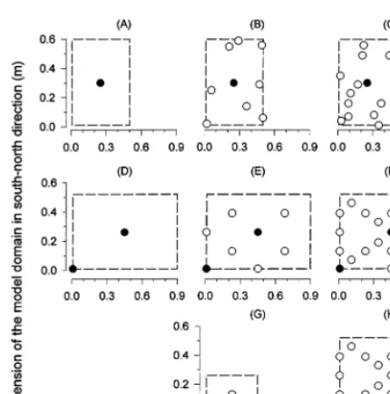
All plants in the model were assumed to have an ellipsoidal foliage envelope and the cube edge length was set to 0.01 m (Ro¨hrig et al., 1999). The latitude of the experimental site (52°15% N)
was input in the model as well as the north – south alignment of the field.
Fig. 1. Distribution of cauliflower ( ) and C. album plants () in the field experiments as repeated in the model. The top and the middle row represent the mixed stands of the cauliflower experiments in 1994 (A – C) and 1995 (D – F), re-spectively. The bottom row shows the pure weed plots in the 1995 experiments (G – H). The columns from left to right represent weed free, low and high weed planting densities.
calculated per layer. Within a layer, a homoge-nous leaf area distribution is assumed, whereas in the vertical dimension a parabolic density func-tion is used. Summafunc-tion over all layers yields the total radiation absorbed by each species.
The modification used here applies to the ex-tinction coefficient for diffuse radiation. Instead of using a constant value, the absorption of solar rays from selected elevation angles in a layer is calculated to be integrated over the hemisphere according to the Gaussian integration procedure (Goudriaan, 1986). Five points, p, are selected at defined distances, d5p, from the central point of
the integration range of the solar elevation angle b. The absorption of radiation originating at these solar heights bp is calculated and weighted, w5p. For the distances and weights for the
Gaus-sian integration see Ro¨hrig et al. (1999), Table 1. The solar elevation angles are determined by:
bp=
p
2(0.5+d5p) for 0Bb5 p 2
with p=[1…5] (11)
The radiation extinction coefficient to be used for integrating the absorption of diffuse radiation is (Goudriaan, 1977, Eq. (2.41)):
Ka=
Oav
sinbp
1−s (12)
where Oav is the average projection of leaves,
which is 0.5 for a spherical leaf angle distribution and sis the scattering coefficient, which amounts to 0.2 for visible radiation. According to the Gaussian integration the relative absorption of diffuse radiation,Fa,f, is then the weighted sum of
all rays considered:
Fa, f=p 2 %
5
p=1
Ip(1−e
−Ka LLY)sinb
pcosbpw5p
(13)
where Ip is the relative irradiance of the selected solar ray, which amounts to 1/p for each solid angle above the canopy and LLY is the total leaf
area in layer LY. Multiplication by sinbp
consid-ers the fraction of radiation effective on a hori-zontal plane and the factor cosbpis needed when
integrating the solid angles over the hemisphere. Since the radiation absorption of canopy with a
2.2.4. Run control
The model runs start at the date of cauliflower transplanting. C. album is initiated at the three-node stage, i.e. at about 300°C days after sowing in the 1994 experiment and at the date of trans-planting in the 1995 experiments. The simulation is terminated when the crop has reached harvest time, which is determined by a specified curd diameter in cauliflower. For those treatments where curds did not reach a marketable size, the model is stopped at the day of the final harvest.
2.2.5. Model simplification
horizontally homogeneous leaf area distribution is insensitive to changes of the solar azimuth angle, the weighted sum has finally to be multiplied by the integration range of both solar angles (2p(p/ 2)=p2). Calculating the absorption of diffuse
radiation in a layer with the above procedure yields a value that is dependent on the leaf area (Goudriaan, 1977) and on the depth in the canopy. Subsequently, the ‘effective’ diffuse radia-tion extincradia-tion coefficient,Kf, is calculated, which
is needed to realise the relative absorption of diffuse radiation given by Eq. (13), thus:
Fa,f=1−e
−Kf LLY
(14)
which can be rewritten as
Kf=
−ln(1−Fa, f)
LLY (15)
Eq. (13) estimates the fraction of absorbed diffuse radiation in relation to the irradiance above the canopy. If the absorption is calculated from the irradiance above a layer I0, LY, Eq. (15) is
modified to give
Kf, LY=
−ln(1−Fa, f/I0, LY)
LLY
(16)
yielding the ‘effective’ diffuse radiation extinction coefficient in a layer Kf, LY, which is used in the
routines of XASSMN.
3. Results and discussion
In general, cauliflower was initially dominant in the canopy becoming increasingly sub-dominant as theC.album grew in time. Evidently, this was more significant when C. album was transplanted compared to a direct sowing to the field. Both species had the same plant height about 60 days after transplanting of cauliflower in 1994, whereas in the 1995 experiments this period was halved. Unless stated otherwise all calibration data were taken from the experiments conducted in 1995 whereas the model was evaluated with data from the trial in 1994.
3.1. Model calibration
3.1.1. Cauliflower
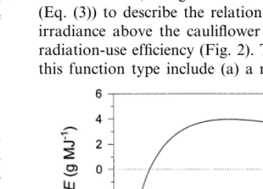
In the second experiment in 1995, the impact of bothC.albumplanting densities on the growth of cauliflower was so substantial, that the crop’s standing biomass decreased. This dry weight re-duction, starting only few weeks after planting, may be attributed to both respiratory losses and to an accelerated senescence and abscission (Spit-ters et al., 1989) due to low radiation. Although senescent leaves were sampled, it cannot be ruled out that part of the biomass shed was already degraded by the time of subsequent harvests. Since no detailed respiration measurements were made, a quantification of the total biomass loss and thus the gross dry weight produced was not possible. Applying the radiation-use efficiency of cauliflower estimated from weed-free plots to sim-ulate growth of weed-infested cauliflower led to a considerable overestimation. To overcome these problems, the net standing biomass is simulated instead of gross dry weights. Furthermore, the radiation-use efficiency showed a considerable seasonal variation between experiments. Pre-sumably due to a lower level of global radiation, the radiation-use efficiency was higher in the sec-ond compared to the first experiment. As a provi-sional measure, a log – normal function was used (Eq. (3)) to describe the relationship between the irradiance above the cauliflower plants and their radiation-use efficiency (Fig. 2). The properties of this function type include (a) a negative function
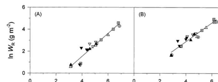
Fig. 3. Relationships between the natural logarithms of (A) root,WR, and shoot dry weight,WSh, and (B) stem,WS, and leaf dry weight,WL, of cauliflower. Symbols denote data are from weed free (Õexp. 1, exp. 2), low (exp. 1,exp. 2) and high ( exp. 1, exp. 2) weed density cauliflower plots. The regressions are: (A) lnWR= −2.67(90.34)+1.05(90.069) lnWSh (r2=0.92); (B) lnW
S= −0.53(90.25)+0.86(90.056) lnWL(r2=0.93). value at low irradiation and after reaching a
maximum (b) a gradual negative slope at high radiation intensities. Thus both the degree of competition as well as the general growing con-ditions could be combined in one relationship. A similar response is obtained by integrating single-leaf photosynthesis (Acock et al., 1978) over the canopy and the diurnal course. The losses predicted by such integration, however, are solely due to respiration whereas the dry matter reduction estimated by Eq. (3) addition-ally includes senescence and abscission. The parameters of the log – normal function were not estimated directly because the equation needs the irradiance above the cauliflower plants (Eq. (4)), which can only be precisely predicted by the model itself. Due to the large number of calculations in the model, the execution time easily exceeds several hours for one simulation run. The parameters were therefore adjusted by eye in repeated model runs with data from all treatments in both 1995 experiments. Measured LAI and plant height of both species were used as input until a good correspondence between the simulation output and measured data was found. Evidently, this procedure is only a stop-gap until further information exists on the pro-duction and degradation of cauliflower biomass under reduced irradiance.
The relationship between the specific leaf area of newly formed leaves of cauliflower and the
radiation environment was established from field experiments with shaded and unshaded plants (Alt, 1999, personal communication). If the PAR above the plants drops below about 2 MJ m−2 day−1, Eq. (9) will predict an
unrealisti-cally high specific leaf area. But this relationship applies to newly produced leaf dry matter only, which is given when a positive radiation-use effi-ciency is predicted, i.e. at an irradiance above c. 1.8 MJ m−2 day−1 (Fig. 2).
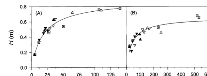
Fig. 4. (A) Relationship between plant height,H, and stem dry weight,WS, and (B) plant diameter,D, and vegetative shoot dry weight, WV, of cauliflower. For the symbol definition see legend of Fig. 3. The regressions are: (A) H=(0.882(90.033)WS)/ (19.49(92.0)+WS) (r2=0.96); (B)D=(0.656(90.32)WV)/(46.31(97.6)+WV) (r2=0.84).
3.1.2. Chenopodium album
The seasonal variation of the radiation-use effi-ciency was also found in C. album but neither planting density nor competition with cauliflower had a significant effect on RUE (Ro¨hrig, 1999). It could furthermore be shown that the root:shoot ratio was constant throughout, but the allometric growth coefficient for leaves and stems increased slightly with planting density. These differences, however, did not affect the accuracy of the simu-lation compared a summary resimu-lationship calcu-lated for all treatments. In order to reduce the number of parameters in the model this general function was used to simulate the stem:leaf ratio in C. album since it could explain about 94% of the variation (Ro¨hrig, 1999). The specific leaf area of C. album was estimated by a linear regression between area and weight of leaves (Fig. 5). Re-gressions calculated separately for all treatments yielded insignificantly different values for SLA. The estimated value (0.0271 m2 g−1) is slightly
higher than the 0.0231 m2 g−1 reported for C.
albumby Kropff and Spitters (1992). All parame-ters estimated for both species are summarised in Table 2.
3.1.3. Simulation results
In weed-free cauliflower plots, the model esti-mated sufficiently well total biomass production, leaf area growth, plant height and the size of the marketable organ (Fig. 6). Calculation of plant height from Eq. (10) resulted in a distinct lag in
height growth after transplanting. This lasted longer in spring than in summer due to slower growth early in the year and may be interpreted as the transplanting shock. Data show that plant height development was even further delayed in the first experiment. In springtime, low tempera-tures may coincide with high irradiances thus dry matter accumulation starts whereas developmen-tal processes are retarded. Since such a tempera-ture effect is not included in the model, plant height is overestimated. Calibration runs revealed problems in reproducing the yield losses in cauliflower due to C. album infestations. These
M
.
Ro
¨hrig
,
H
.
Stu
¨tzel
/
Europ
.
J
.
Agronomy
14
(2001)
13
–
29
23
Overview of the parameter estimates for cauliflower andC.album(values in parentheses denote S.E.)
C.album Cauliflower
Parameter
1994 1995
1994 1995 1995 1995
experiment 2 experiment 1
experiment 2 experiment 1
109 123 201
Day of planting/sowing (day) 108 114 199
–
200 200 – –
Curd diameter at harvest (mm) 200
– – –
Day of final harvest (day) 171 191 282
Radiation-use efficiency, Fig. 2 Fig. 2 Fig. 2 3.5 3.14 (90.036)a 4.34 (90.12)a
RUE (g MJ−1)
Eq. (9) Eq. (9) Eq. (9) Fig. 5b Fig. 5b
Specific leaf area, SLA (m2g−1) Fig. 5b
−2.13 (90.12)a
Root–shoot allometry,a Fig. 3A Fig. 3A Fig. 3A −2.13 (90.12)a −2.13 (90.12)a
1.06 (90.021)a 1.06 (90.021)a
1.06 (90.021)a
Root–shoot allometry,b
−1.42 (90.25)a
Fig. 3B Fig. 3B Fig. 3B −1.42 (90.25)a −1.42 (90.25)a
Stem–leaf allometry,h
1.52 (90.058)a
1.52 (90.058)a 1.52 (90.058)a
Stem–leaf allometry,g
0.0005 0.0005 0.0005 – –
Translocation rate,rt(°C−1) –
f(L,Tav)a
Plant height,H(m) Fig. 4A Fig. 4A Fig. 4A f(L,Tav)a f(L,Tav)a
f(Tav, planting
Fig. 4B
Plant diameter,D(m) Fig. 4B Fig. 4B f(Tav, planting f(Tav, planting
density)a
density)a density)a
aFor details see text and Ro¨hrig (1999).
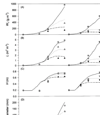
Fig. 6. Simulated (lines) and observed values (symbols) for (A) total dry weight,WT, (B) leaf area index,L, (C) plant height,H, and (D) curd diameter of cauliflower. Data are from weed free (Õexp. 1, exp. 2, solid line), low (exp. 1,exp. 2, dotted line) and high (exp. 1,exp. 2, dashed line) weed density cauliflower plots.
losses were only simulated correctly if observed values for LAI of C. album were given as input. With this prerequisite, total dry weight of cauliflower was slightly overestimated in the first experiment whereas the almost complete yield loss in the second experiment (Fig. 6A) was ade-quately reproduced. This is due to a more accu-rate simulation of plant height of cauliflower in the summer compared to the spring experiment. The size of the marketable organ was calculated sufficiently accurately in all treatments. In the weed-infested plots of experiment 2, the curd dry
weight and diameter increased with a decreasing total growth rate. Cauliflower plants evidently attempt to initiate, maintain and develop an infl-orescence even under unfavourable growing con-ditions, which can be explained by retranslocation of dry weight from vegetative to reproductive plant organs.
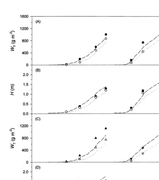
the LAI as input, total dry matter production ofC.
albumwas nevertheless underestimated in the first cauliflower experiment, whereas simulation results are better in the second experiment (Fig. 7A and C). This indicates that the radiation-use efficiency ofC. album(Ro¨hrig, 1999) may not be estimated correctly, requiring further data. The approach used to calculate of plant height ofC.albumyielded an acceptably accurate simulation (Fig. 7B and D). The limitation of the model is that it does not give correct results, if the LAI of C. album is calculated dynamically. Underestimating the total
growth of C.albumlike in the first experiment in 1995, results in a slower leaf area development. As plant height is assumed a function of LAI, plants are simulated to be smaller. Leaf area and plant height, however, mainly determine the competitive-ness of a plant species with respect to PAR inter-ception. Underrating these determinants results in an unrealistic low impact of C. album on cauliflower. The model is therefore particularly sensitive to leaf area development, an aspect that has to be reconsidered in future model improvements.
Fig. 7. Simulated (lines) and observed values (symbols) for (A, C) total dry weight,WT, and (B, D) plant height,H, ofC.album. Data are from pure weed stands (A, B;, exp. 1,,exp. 2) and mixed stands with cauliflower (C, D;,exp. 1,,
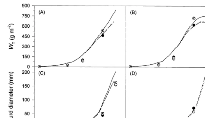
Fig. 8. Simulated (lines) and observed values (symbols) from the 1994 cauliflower experiment used for evaluation. Symbols denote weed free (Õ, solid line), low (, dotted line) and high ( , dashed line) weed density cauliflower plots. (A – C) Total dry weight,
WT, leaf area index,L, and curd diameter of cauliflower, respectively, and (D) total dry weight,WT, ofC.album.
3.2. Model e6aluation
The late emergence of C. album due to low spring temperatures and a long juvenile phase resulted in a delayed onset of competition in the 1994 cauliflower experiment (Fig. 8). Only minor differences between both weed densities were found, which are adequately reproduced by the model with respect to total dry weight and leaf area index of cauliflower. Although, curd growth is slightly overestimated, the model correctly ter-minated the calculations at the measured harvest date. Dry matter production ofC.albumwas also simulated appropriately by calculating the leaf area development dynamically and using an aver-age radiation-use efficiency of 3.5 g MJ−1. This
value was estimated from the 1995 results and is supported by Kiniry et al. (1992), who derived RUE values for C3weed species ranging from 3.3
to 3.7 g MJ−1
. The simulation results presented give a first indication to the applicability of the relationships and assumptions used. The model is able to predict the reduced curd yield of cauliflower by late weed infestations. It thus re-produces the high competitiveness of this crop with regard to radiation interception. It has to be
noted, however, that the 1994 cauliflower data set is incomplete making a further evaluation necessary.
3.3. Model simplification
At the outset of model simplification, a com-parison between the complex and the simplified model under identical conditions was made. As-suming a ‘closed canopy’ situation, both models were run to simulate the weed-free cauliflower plots of the 1995 experiments. The relationship between the PAR absorption calculated by the complex model and by the simple model was very close (slope=1.0001, r2\0.999), deviations
Fig. 9. Relationship between the deviation in the calculation of radiation absorption between complex and simplified model and the relative ground cover,rgc. Symbols denote simulated radiation absorption from weed free cauliflower plots from experiment 1 (Õ) and experiment 2 ( ). The regression is
Ia, complex/Ia, simple=
0.77(90.0053)+0.28(90.007)(1−e−1.65 (90.15)rgc) (r2=0.96)
cauliflower experiments in 1995 (Fig. 9). For the simulation of mixed canopies, the relative ground cover of both species is summed. Furthermore, the calculation of I0, c (Eq. (4)) had to be
modified, since the radiation absorbed by the taller species is overestimated if a homogeneously distributed leaf area is assumed. As an approxi-mation, the leaf area in the upper layer is assumed to have an average relative ground cover of 50%. Eq. (18) then yields a value of c. 0.93, thus Eq. (4) is modified to
I0,S=I0−0.93(Ia, t−Ia,HS) (19)
The relationships in Eqs. (18) and (19) were evalu-ated by simulation of mixed stands. A comparison of simulation results in different competitive envi-ronments from both models reveals a good corre-spondence (Table 3). The variation between the models increases, however, with canopy hetero-geneity. In the second cauliflower experiment, the crop was suppressed to such an extent, that the plants stayed comparatively small leading to a continuously heterogeneous canopy. In other treatments, the canopy structure approaches ho-mogeneity in the course of time and the error made by the simplified model is less significant for the final result. A scenario calculation for 1 day showed that a reduction in weed density and thus a higher spatial heterogeneity of the canopy leads to an increased deviation of the simplified model (Table 4). The deviation is reduced by introduc-tion of Eq. (18) but it still does not completely account for the variation. Furthermore, the weed and that a value of 1.0 is not exceeded, the
relative ground cover is approximated by
rgc=min
D2p4PD, 1.0
(17)whereD(m) is the plant diameter and PD (m−2)
is the planting density. This is then related to the deviation between the complex and the simplified model by
Ia, complex
Ia, simple
=c1+c2(1−e
−c3rgc) (18)
wherec1,c2 andc3are calibration factors with c1
representing the intercept. The parameters were estimated using the weed-free plots of both
Table 3
Comparison of the cumulative radiation absorption and total dry weight of cauliflower in the 1995 experiments between the complex (CM) and the simplified model (SM)a
Cumulative radiation absorption
Experiment/treatment Total dry weight
SM (MJ m−2)
CM (MJ m−2) SM/CM (%) CM (g m−2) SM (g m−2) SM/CM (%)
1/weed free 326.7 328.8 101 907.5 910.4 100
1/low weed density 147.0 143.8 98 486.2 474.8 98
107 261.5
245.5 108
1/high weed density 83.0 89.4
845.7
253.8 254.7 100 842.6 100
2/weed free
69.7
66.9 105
2/low weed density 104 138.8 145.4
128 83.3
65.2 135
42.6 2/high weed density 31.5
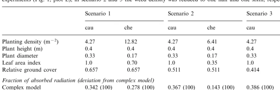
Table 4
Sensitivity analysis for the simplified model. Scenario 1 represents the situation in a low weed density plot in the 1995 cauliflower experiments (Fig. 1, plot E), in scenario 2 and 3 the weed density was reduced to one half and one sixth, respectivelya
Scenario 2 Scenario 3 Scenario 1
che cau
cau che cau che
12.82 4.27 6.41 4.27
Planting density (m−2) 4.27 2.14
0.4 0.4 0.4
0.4 0.4
Plant height (m) 0.4
0.33
Plant diameter 0.17 0.33 0.17 0.33 0.17
Leaf area index 1.0 0.70 1.0 0.35 1.0 0.117
0.657 0.511 0.511 0.414
0.657 0.414
Relative ground cover
Fraction of absorbed radiation(de6iation from complex model)
0.278 (100) 0.367 (100) 0.143 (100) 0.386 (100) 0.049 (100) Complex model 0.342 (100)
0.277 (99) 0.441 (120) 0.155 (108)
0.395 (116) 0.478 (124)
Uncorrected simple model 0.056 (113)
0.264 (95)
Corrected simple model 0.378 (110) 0.410 (112) 0.144 (100) 0.434 (112) 0.051 (103) aShown are the fractions of absorbed radiation by cauliflower (cau) andC.album(che) as calculated by the complex model and the simple model. For the latter, results are given before (uncorrected) and after (corrected) modification by Eq. (18). Calculations were made for day 152 (1 June) at 50% diffuse radiation.
densities used in the cauliflower experiments led to a substantial yield reduction up to a complete loss. Thus in vegetable production, much lower weed densities will be of particular interest. In this case, the complex model will give more accurate information on the radiation distribution between crop and weeds.
4. Conclusion
In summary, simulation results encourage the use of a three-dimensional radiation interception model when the leaf area is not homogeneously distributed in the canopy. Even if a mainly one-di-mensional approach is modified by a correction factor, deviations still persist due to the complex system of interactions between the spatial leaf area distribution of competing species and the radiation environment. The present findings sug-gest that a closer look at dry matter production and losses under low radiation in cauliflower is required and also indicate uncertainties in the quantification of growth processes in C. album. Nevertheless, the model promises to be an effec-tive tool to gain insight into the mechanisms of radiation competition and thus support decision-making in weed-control management.
Acknowledgements
Financial support through the Deutsche Forschungsgemeinschaft (DFG) is gratefully acknowledged.
References
Acock, B., Charles-Edwards, D.A., Fitter, D.J., Hand, D.W., Ludwig, L.J., Wilson, J.W., Withers, A.C., 1978. The contribution of leaves from different levels within a tomato crop to canopy net photosynthesis: an experimental exami-nation of two canopy models. J. Exp. Bot. 29, 815 – 827. Angus, J.F., Cunningham, R.B., Moncur, M.W., Mackenzie,
D.H., 1981. Phasic development in field crops. I. Thermal response in the seedling phase. Field Crops Res. 3, 365 – 378.
Cousens, R.D., Brain, P., O’Donovan, J.T., O’Sullivan, A., 1987. The use of biologically realistic equations to describe the effects of weed density and relative time of emergence on crop yield. Weed Sci. 35, 720 – 725.
Debaeke, P., Caussanel, J.P., Kiniry, J.R., Kafiz, B., Mondragon, G., 1997. Modelling crop:weed interactions in wheat with ALMANAC. Weed Res. 37, 325 – 341. Goudriaan, J., 1977. Crop Micrometeorology: A Simulation
Study. Pudoc, Wageningen.
Goudriaan, J., 1986. A simple and fast numerical method for the computation of daily totals of crop photosynthesis. Agric. For. Meteorol. 38, 249 – 254.
Hewson, R.T., Roberts, H.A., 1973. Effects of weed competi-tion for different periods on the growth and yield of red beet. J. Hortic. Sci. 48, 281 – 292.
Kage, H., Stu¨tzel, H., 1999. A simple empirical model for predicting development and dry matter partitioning in cauliflower (Brassica oleraceaL.botrytis). Sci. Hortic. 80, 19 – 38.
Kiniry, J.R., Williams, J.R., Gassman, P.W., Debaeke, P., 1992. A general, process-oriented model for two competing plant species. Trans. ASAE 35, 801 – 810.
Kropff, M.J., Spitters, C.J.T., 1991. A simple model of crop loss by weed competition from early observations of rela-tive leaf area of the weeds. Weed Res. 31, 97 – 105. Kropff, M.J., Spitters, C.J.T., 1992. An eco-physiological
model for interspecific competition, applied to the influence ofChenopodium albumL. on sugar beet. I. Model descrip-tion and parameterizadescrip-tion. Weed Res. 32, 437 – 450. Kropff, M.J., Lotz, L.A.P., Weaver, S.E., 1993. Practical
applications. In: Kropff, M.J., van Laar, H.H. (Eds.), Modelling Crop – Weed Interactions. CAB International, pp. 83 – 104.
Lorenz, H.P., Schlaghecken, J., Engel, G., Maync, A., Ziegler, J., 1989. Ordungsgema¨ße Stickstoffversorgung im Frei-landgemu¨sebau nach dem kulturbegleitenden Nmin – Sollw-erte – (KNS) System. Ministerium fu¨r Landwirtschaft, Weinbau und Forsten, Rheinland-Pfalz, Mainz.
Lotz, L.A.P., Kropff, M.J., Bos, B., Wallinga, J., 1992. Predic-tion of yield loss based on relative leaf cover of weeds. In: Proceedings 1st International Weed Control Congress, pp. 290 – 296.
Manrique, L.A., Kiniry, J.R., Hodges, T., Axness, D.S., 1991. Dry matter production and radiation interception of potato. Crop Sci. 31, 1044 – 1049.
Nieto, J.H., Brondo, M.A., Gonzales, J.T., 1968. Critical periods of the crop growth cycle for competition from weeds. PANS. (C) 14, 159 – 166.
Persall, W.H., 1927. Growth studies. VI. On the relative sizes of growing plant organs. Ann. Bot. 41, 549 – 556. Qasem, J.R., 1992. Pigweed (Amaranthusssp.) interference in
transplanted tomato (Lycopersicon esculentum). J. Hortic. Sci. 67, 421 – 427.
Roberts, H.A., 1976. Weed competition in vegetable crops. Ann. Appl. Biol. 83, 321 – 324.
Ro¨hrig, M., Stu¨tzel, H., Alt, C., 1999. A three-dimensional approach to modeling light interception in heterogeneous canopies. Agron. J. 91, 1024 – 1032.
Ro¨hrig, M., 1999. Modelling the light competition between crops and weeds. University of Hannover, Hannover, Ger-many Ph.D. thesis.
Spitters, C.J.T., Aerts, R., 1983. Simulation of competition for light and water in crop – weed associations. Asp. App. Biol. 4, 467 – 483.
Spitters, C.J.T., van Keulen, H., van Kraalingen, D.W.G., 1989. A simple and universal crop growth simulator:
SU-CROS87. In: Rabbinge, R., Ward, S.A., van Laar, H.H. (Eds.), Simulation and System Management in Crop Pro-tection. Pudoc, Wageningen, pp. 147 – 181.
Spitters, C.J.T., 1989. Weeds: population dynamics, germina-tion and competigermina-tion. In: Rabbinge, R., Ward, S.A., van Laar, H.H. (Eds.), Simulation and System Management in Crop Protection. Pudoc, Wageningen, pp. 182 – 392. Spitters, C.J.T., 1990. On descriptive and mechanistic models
for inter-plant competition, with particular reference to crop – weed interaction. In: Rabbinge, R., Goudriaan, J., van Keulen, H., Penning de Vries, F.W.T., van Laar, H.H. (Eds.), Theoretical Production Ecology: Reflections and Prospects. Pudoc, Wageningen, pp. 217 – 236.
Stu¨tzel, H., Aufhammer, W., 1991. Dry matter partitioning in a determinate and indeterminate cultivar ofVicia fabaL. under contrasting plant distributions and densities. Ann. Bot. 67, 487 – 495.
Stu¨tzel, H., Charles-Edwards, D.A., Beech, D.F., 1988. A model of partitioning of new above-ground dry matter. Ann. Bot. 61, 481 – 487.
Stu¨tzel, H., 1995a. A simple model for simulation of growth and development in faba beans (Vicia fabaL.) 1. Model description. Eur. J. Agron. 4, 175 – 185.
Stu¨tzel, H., 1995b. A simple model for simulation of growth and development in faba beans (Vicia fabaL.) 2. Model evaluation and application for the assessment of sowing date effects. Eur. J. Agron. 4, 187 – 195.
Thornley, J.H.M., Johnson, I.R., 1990. Plant and Crop Mod-elling. Oxford University Press, New York.
van Keulen, H., Penning de Vries, F.W.T., Drees, E.M., 1982. A summary model for crop growth. In: Penning de Vries, F.W.T., van Laar, H.H. (Eds.), Simulation of Plant Growth and Crop Production. Pudoc, Wageningen, pp. 87 – 97.
Weaver, S.E., 1984. Critical period of weed competition in three vegetable crops in relation to management practices. Weed Res. 24, 317 – 325.
Wiebe, H.J., 1979. Short term forecasting of the market supply of vegetables, especially cauliflower. Acta Hortic. 97, 399 – 409.
Wilkerson, G.G., Jones, J.W., Boote, K.J., Ingram, K.T., Mishoe, J.W., 1983. Modeling soybean growth for crop management. Trans. ASAE 26, 63 – 73.
Wilkerson, G.G., Jones, J.W., Coble, H.D., Gunsolus, J.L., 1990. SOYWEED: a simulation model of soybean and common cocklebur growth and competition. Agron. J. 82, 1003 – 1010.
Williams, J.R., Jones, C.A., Kiniry, J.R., Spanel, D.A., 1989. The EPIC crop growth model. Trans. ASAE 32, 497 – 511. Wurr, D.C.E., Fellows, J.R., Sutherland, R.A., Elphinstone, E.D., 1990. A model of cauliflower curd growth to predict when curds reach a specified size. J. Hortic. Sci. 65, 555 – 564.