Children, and Intergenerational
Mobility
Comparing Sons of Foreign- and Native-Born
Fathers
Christian Dustmann
a b s t r a c t
This paper studies parental investment in education and intergenerational earnings mobility for father-son pairs with native- and foreign-born fathers. We illustrate within a simple model that for immigrants, investment in their children is related to their return migration probability. In our empirical analysis, we include a measure for return probabilities, based on repeated information about migrants’ return intentions. Our results suggest that educational investments in the son are positively associated with a higher probability of a permanent migration of the father. We also find that the sonÕs permanent wages are positively associated with the probability of the father’s permanent migration.
I. Introduction
Immigrants contribute significantly to the overall economic perfor-mance of their host economies. It is therefore not surprising that a large literature is concerned with the earnings mobility of the foreign-born population, both in iso-lation, as well as in comparison with those who are native-born.1But immigrants not only have an immediate effect on wealth accumulation and earnings and skill com-position. They transmit their earnings status, as well as socioeconomic and cultural characteristics to the next generation. The economic adjustment process within the
Christian Dustmann is a professor in the department of economics at University College, London. He is grateful to David Card for many helpful discussions, and to Jerome Adda, Teresa Casey, Steve Machin, Gary Solon, and two anonymous referees for comments. This research was funded by the Economic and Social Research Council (grant RES-000-23-0332). The data on which this analysis is based are available from the DIW in Berlin. Users must register and sign an agreement with the data provider. The author will help other researchers in pursuing these data. He may be contacted through Department of Economics, University College, London, Gower Street, London WC1E. Email: c.dustmann@ucl.ac.uk [Submitted July 2006; accepted April 2007]
ISSN 022-166X E-ISSN 1548-8004Ó2008 by the Board of Regents of the University of Wisconsin System
T H E J O U R NA L O F H U M A N R E S O U R C E S d X L I I I d 2
immigrant’s own generation has long been recognized as an important step in under-standing the economic effects of immigration. In underunder-standing the long-term con-sequences of immigration, assessment of intergenerational mobility in immigrant communities is perhaps equally important.
Although the process of intergenerational economic mobility has been intensively studied for majority populations (see among others Solon 1992; Zimmermann 1992; Bjørklund and Jaentti 1997; Plug 2004; Bjørklund, Lindahl, and Plug 2006; see Solon 1999, 2002 for reviews), less is known about intergenerational transmission in immigrant communities. For the United States, early studies by Chiswick (1977) and Carliner (1980) compare earnings of immigrants with their descendants and their children. More recently, Borjas (1992, 1994) emphasizes that intergenerational eco-nomic mobility among immigrants may be more complex. He argues that estimating the usual models of intergenerational income mobility may miss out an important as-pect of this process: The skills of the next generation may not only depend on parental inputs, but also on the quality of the ethnic environment of the parent generation. Bor-jas terms this ‘‘ethnic capital.’’ In later work BorBor-jas (1995) shows that one reason for the external effects of ethnicity is segregation into particular neighborhoods—a point that has been reemphasized in work by Nielsen, Rosholm, Smith, and Husted (2001). This paper focuses on another important characteristic of immigrant communities that may affect the process of intergenerational mobility: The probability the immi-grant attaches to a permanent migration as opposed to a future return to the home country. A number of papers show that return migration may affect different aspects of immigrants’ behavior. Work by Galor and Stark (1990) suggest that positive return probabilities may affect savings behavior. Dustmann (1997) provides evidence that married immigrant women whose husbands plan to return to their home countries have a higher labor force participation rate. Dustmann (1999) develops a model that suggests that immigrants who have higher probabilities of returning are less likely to acquire human capital specific to the host country economy if this human capital has a lower return back home. He finds evidence for this by investigating their invest-ment in language skills. In a recent paper, Cortes (2004), arguing along the same lines, explains the higher rate of human capital accumulation by refugee immigrants in the United States with lower probabilities of their return migration.
Similar considerations may hold in an intergenerational context. In this paper, we investigate how parental probabilities of a permanent, as opposed to a temporary, mi-gration affect investment in their children’s education and intergenerational earnings mobility. We develop a model of intergenerational mobility with parental invest-ments in the childÕs earnings potential, based on previous work by Becker and Tomes (1979) and Solon (2004), which we extend by allowing the probability of a perma-nent migration to affect parental human capital investments. The model suggests that, if returns to educational investment undertaken in the host country, are higher in the host than in the home country, and if the parent believes that the child’s return probability increases in his own, educational investments should increase with the permanent migration probability, as should the childÕs permanent earnings.
To understand the precise nature of how parental background may affect earnings in the next generation, we commence by estimating investment equations, relating educational investments to parental earnings, as well as return probabilities. We find strong and consistent evidence that, for immigrants, parental investment in education increases with the permanent migration probability. Estimation of investment equa-tions that relate educational achievements to permanent parental earnings show esti-mates of similar magnitude for immigrants and natives. For earnings mobility, we again find that the son’s permanent earnings increase in the fatherÕs permanent mi-gration probability, conditional on father’s permanent earnings and education.
We also find that educational achievements of immigrant parents are not correlated with educational achievements of their children. This is in contrast with previous work by Card, DiNardo, and Estes (1998) for the United States, who show that much of the intergenerational link between the economic status of immigrant fathers and their sons and daughters works through education.2Our findings are in line with sim-ilar results reported by Gang and Zimmermann (2000). One explanation for this weak link in educational outcomes for immigrants is that it is the permanent earnings position of the father that matters for the son’s educational attainment; the fatherÕs education is then only correlated with the son’s education if education is a good pre-dictor for earnings. We show that this is not the case for immigrants in our sample.
We also estimate intergenerational mobility coefficients. Our analysis extends some previous work on Germany by Couch and Dunn (1997) and Wiegand (1997) for the native-born, but provides more robust estimates based on a longer panel, allowing us to address the problem of measurement error in permanent parental earn-ings, which bedevils studies of intergenerational transmission (see Solon 1989). In addition, we distinguish between immigrant and native father-son pairs. Our results reveal that intergenerational mobility between native-born fathers and their sons is larger than between foreign-born fathers and their sons, conditional on return prob-abilities of foreign-born fathers, although the difference is not statistically significant. The paper is structured as follows. In the next section we develop a theoretical model, and discuss its empirical implications. In Section III we describe the data and the sample. Section IV presents the results, and Section V concludes.
II. Theory
Our model is a permanent income model of intergenerational mobil-ity with parental investments in the child’s earnings potential, following early work by Becker and Tomes (1979) and Solon (2004). It extends Solon (2004) by taking account of the way the probability of a permanent migration as opposed to a future return, may affect the decision of the parent to invest in their offspringÕs human capital. We consider a one-person household with one child. There are two periods. In the first period (Period 0) both parent and child live in the host country. In the second period (Period 1), the parent returns to the home country with probability 1 -p, and remains in the host country with probabilityp. The parent retires in Period 1,
and has earnings in Period 0 equal toY0. The child is in full-time education in Period
0, and participates in the labor market in Period 1, either in the parent’s home coun-try, or in the host country.
The parent is altruistic and maximizes an intertemporal utility function, by choos-ing first period savchoos-ingss0, and investment in the child’s human capital in the first
pe-riod,I0. When making these choices, the parent attaches the same probability p to his
childÕs location choice in the second period as to his own. This assumption simplifies the algebra, but can be relaxed without affecting the key implications of our model, as long as the parent perceives the child’s probability to remain in the host country to increase in his own probability of remaining.
The parent’s intertemporal utility function is given by
V¼uðc0Þ+p½uðcI1Þ+gvðyI1Þ+ð12pÞ½uðcE1;bÞ+gvðyE1Þ ð1Þ
whereu(.) andv(.) are the parent’s and the childÕs utility functions, defined over pa-rental consumption in Period 0c0, and parental consumption and the child’s earnings
in Period 1, andcJ
1andyJ1. HereJ¼E;Istands for Emigration or Immigration
coun-try. The parametergis an altruistic weight. Ifg¼0, the parent does not consider the childÕs welfare in Period 1. The parameterbis a preference parameter, reflecting a preference for consumption at home over consumption abroad. Ifb> 1, more utility is obtained from consuming in the home country as compared to the host country.
We assume that parental investments translate into human capital of the child (h1)
according to the following production technology:
h1¼ulogI0+e0: ð2Þ
The parameteruis a technology parameter measuring the productivity of invest-ments. The terme0is the human capital the child receives without any direct parental
investments (see Becker and Tomes 1979; Solon 2004 for a similar formulation). This term represents the attributes endowed upon the child, depending on character-istics of the parent, the child’s upbringing, genetic factors, environment, and luck. It also may depend on existing networks, as well as the lack of opportunity to move out of social and economic structures from one generation to the next. This latter factor may be particularly important for immigrants, and we will discuss its implications later. It includes what Borjas (1992) calls ‘‘ethnic capital’’—the quality of the envi-ronment in which parental investments are made.
Human capital translates into earnings according to the following relationship:
logyj1¼mj+rjh1; ð3Þ
wherej¼I;E. Our formulation allows for different base wagesmj
, as well as dif-ferent returns to the child’s human capital rjin the two countries. It follows from Equations 2 and 3 that the childÕs earnings in the second period are related to parental investments as:
logyj1¼mj+rjulogI0+rje0 ð4Þ
The parent’s consumption in Period 0 equals c0¼Y0- I0- s0, where Y0is first period
for the child’s earnings into Equation 1, the optimization problem of the parent can
Maximizing Equation 5 with respect to savings and investment, and solving the first order conditions for the optimal investmentI0yields:
I0¼
guðprI +ð12pÞrEÞ
guðprI+ð12pÞrEÞ+ð1 +p+bð12pÞÞY0
¼Gðp;rE;rI;b;g;uÞY0: ð6Þ
The term in the numerator, which is equal to the first term in the denominator, is the expected utility gain to one log unit of parental investment in the child’s human cap-ital. The second term in the denominator is the expected lifetime utility from one log unit of additional consumption.
Simple comparative statics show that investment in the child’s human capital increases in p, the probability of a permanent migration, as long as the return to human capital investments is higher in the host country (rI>rE). Furthermore, a lower proba-bility of a permanent migration increases the expected gain in utility by consuming in the home country, as long asb> 1: The parent prefers to save more resources for their own future consumption, thus reducing investment in the child. The combined effect leads to an increase in investment with the probability of a permanent migration. Finally, investment increases with altruismgand productivity of investmentu.
An estimable version of Equation 6 is obtained by taking logs, and adding an error term:
logEdi¼a1+a2Pi0+X#ia+blogyi0+ei;
ð7Þ
whereEdiis a measure of child’s educational attainment,Pis a variable measuring
the probability of a permanent migration,Xare additional control variables, and y0
are permanent earnings of the father. Below we test whether investment into child-renÕs education increases with the probability of a permanent migration. IfrI>rE,we should expecta2to be positive.
Now consider the relationship between the child’s earnings and the parentÕs earn-ings for children who are observed in the host country in Period 2. Substituting Equa-tion 6 into EquaEqua-tion 4 and rearranging terms yields:
logyI1¼mI+rIulogG+rIulogY0+rIe1: ð8Þ
Equation 8 is similar to the relationship between son’s earnings and fatherÕs earn-ings, as derived in Solon (1999, 2004), except for the term Gwhich, as we show above, increases in the probability of a permanent migration. An estimable version of Equation 8 is given by:
logyi1¼a1+a2Pi0+ +
K
k¼1
a3kDik0+blogyi0+ei0;
ð9Þ
variablesDik0are dummy variables for the origin countrykof individuali’s father.
They capture, among other factors, differences in ethnic capital (see Borjas 1992).3 Again, ifrI>rE,a2should be positive. We will test for this below.
III. Background, Data, and Descriptives
A. Background
Between the mid 1950s and 1973, the strong economic development in Northern Europe and the resulting demand for labor, led to a large inflow of immigrants mainly from the periphery countries of Europe, but also from Turkey, North Africa, South America, and Asia. The main receiving countries were Belgium, France, Germany, the Netherlands, Switzerland, and the Scandinavian countries.
The West-German economy experienced a strong upward swing after 1955, ac-companied by a sharp fall in the unemployment rate (between 1955 and 1960, the unemployment rate fell from 5.6 percent to 1.3 percent) and an increase in labor demand. This generated a large immigration of workers from Southern European countries and Turkey into Germany. The percentage of foreign-born workers employed in West Germany increased from 0.6 percent in 1957 to 5.5 percent in 1965, to 11.2 percent in 1973, and declined thereafter. Bilateral recruitment agree-ments were set up between Germany and Italy, Spain, Greece, Turkey, Portugal, and Yugoslavia in the 1950s and 1960s.
Labor migration over this period was initially considered as temporary by both the immigration countries and the emigration countries. Individuals were not expected to settle permanently. The German recruitment policy was based on the assumption that foreign workers would after some years return to their home countries. Still, although return migration has been quite considerable (see Bohning 1987), a large fraction of foreign-born workers settled permanently.
1. The Data and Sample
The data we use for this analysis stem from 19 waves of the German Socio-Eco-nomic panel (GSOEP 1984-2002), which is a household-based panel survey, similar to the U.S. Panel Study of Income Dynamics (PSID) or the British Household Panel Study (BHPS). Initiated in 1984, the GSOEP oversamples the then resident immi-grant population in Germany, which stems from the migration movement we have described above. In the first wave, about 4,500 households with a German born household head were interviewed, and about 1,500 households with a foreign-born household head. The data are unique in providing repeated information on a boost sample of immigrants over a long period of time. For our analysis, we use observa-tions of the foreign-born from the over-sample, as well as from the standard sample. Each individual in a household and over the age of 16 is interviewed. The house-hold head provides information about all other individuals in the househouse-hold and be-low the interviewing age. Individuals who leave households and form their own households are included in the panel. When individuals are 16 years old, they receive
their own personal identifier, and pointers connect them to their mother and their father. We construct a sample of father-son pairs for foreign-born and native-born fathers. We define a second generation immigrant as an individual who is born in Germany, and whose father is born abroad. The definition of our sample is in the tradition of previous studies on intergenerational mobility based on the PSID (see, for example, Solon 1992).4Our reference group includes individuals who are likewise born in Germany, and whose father is German born. In our analysis we use only father-son pairs.5
We analyze below the relationship between permanent migration probabilities, permanent parental earnings, and investment into sons’ education. We also analyze intergenerational earnings mobility, and how the sonÕs permanent wages relate to the father’s permanent migration probability. Our analysis of educational achieve-ments considers secondary track choice. Track choices in Germany are made at the age of 10, and determine whether individuals will be entitled to study at univer-sity, or will receive secondary education that entitles them only for vocational or apprenticeship based post-secondary education. Secondary track choice is strongly correlated with later earnings (see Dustmann 2004). For this analysis, we include all sons above the age of 16, as their track choice has already been made, even if they are still in secondary education. We also analyze completed education, and discuss results briefly in the text. Here we use only individuals above the age of 20, and who have completed education. For the analysis on earnings mobility, we exclude sons who are younger than 20 years; our age range is between 20 and 34.
2. Sample Characteristics and Variables
Our resulting samples contain a total of 795 sons born to native-born fathers, and 334 sons of foreign-born fathers. Because some fathers have more than one son, we have 640 corresponding native-born fathers, and 251 foreign-born fathers. In Table 1, we provide a breakdown of fathers and sons in the two samples.
In Table 2, we display information on the fathers’ observable characteristics. For-eign-born fathers have about two years less education than native-born fathers do. The age of fathers when the son was born is similar, at about 30 years. Foreign-born fathers were on average in Germany for 5.5 years when their son was born.
As a measure for earnings, we use real hourly log wages for both fathers and sons. The GSOEP provides information on average monthly gross earnings in the month preceding the interview, and on actual weekly hours worked for pay during that month. From that information, and using a consumer price index, we compute an hourly real log wage rate in 2002 prices.
A common problem in the literature on intergenerational mobility is the lack of suf-ficient information for the estimation of a permanent wage for fathers as well as their sons, which is particularly severe in short panels. Zimmerman (1992), Solon (1989, 1992), and Dearden et al. (1997) among others, emphasize the problems of
measurement error in parental earnings for the estimation of intergenerational mobility parameters. The length of our panel allows us to address this problem. Appendix Table A1 displays valid wage spells of fathers in our sample, where the first set of columns report numbers for foreign-born fathers and the second set of columns for native-born fathers.
An individual can report earnings a total of 19 possible years, corresponding to a total of 2,577 earnings spells for foreign-born fathers, and a total of 7,262 earnings spells for native-born fathers. About 75 percent of fathers in the two samples have more than six wage observations, constituting, for each group, more than 90 percent of all wage spells in the data.
For sons, we disregard earnings spells while being on apprenticeship schemes. Ap-prenticeship schemes are vocational training schemes that pay low and regulated wages, and these wages are not appropriate measures for permanent earnings status. As stated above, we also exclude wage spells when individuals were younger than 20, for similar reasons. Appendix Table A2 displays the wage information for sons. Table 1
Foreign-Born and Native-Born Fathers
Foreign-Born Fathers Native-Born Fathers
Number of Sons to Father Number Percent Number Percent
1 182 72.51 500 78.13
2 55 21.91 126 19.69
3 14 5.58 13 2.03
4 — — 1 0.16
Total number of fathers 251 100.00 640 100.00
Total number of sons 334 795
Source: GSOEP, various years
Table 2
Individual Characteristics, Fathers
Foreign-Born Fathers Native-Born Fathers
Mean
Standard
Deviation Mean
Standard Deviation
Years of education, father 9.2 1.9 11.7 2.6
Age father when child born 30.6 6.3 30.0 6.2
Years since migration when child born
5.6 5.5 — —
Among those with foreign-born fathers, there are 161 individuals with 606 valid wage spells; among those with native-born fathers, there are 373 individuals with 1,824 valid wage spells.
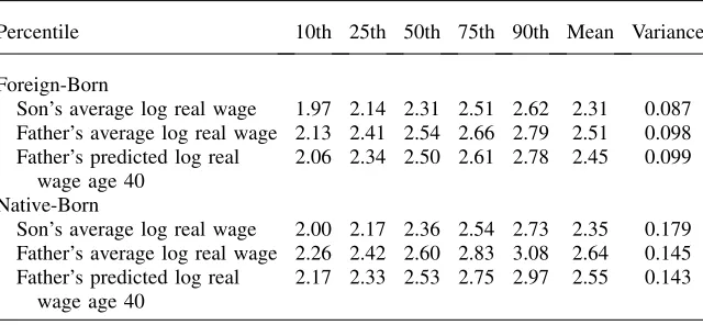
In Table 3 we display percentiles as well as the mean and variance of average log real wages in our data. The entries in the table show that mean wages of native-born fathers are about 13 percent higher than mean wages of foreign-born fathers. For sons, this dif-ference has reduced to 4 percent. Wages of both sons and fathers in the native sample are considerably more dispersed than wages of sons and fathers in the sample of foreign-born fathers. For natives, earnings of sons are slightly more dispersed than earnings of fathers—similar to the findings of U.S. studies using similar data (see Solon 1992). For the foreign-born, however, fathersÔearnings seem to be more dispersed than sonsÕ earn-ings. Differences between sons of native- and foreign-born fathers seem to be similar throughout the distribution, while differences for native- and foreign-born fathers are slightly more substantial in the upper percentiles of the distribution.
a. Permanent Earnings
To eliminate measurement error, we essentially follow the literature, which averages wages over a number of years, thus increasing the signal-noise ratio in earnings information (see for example Solon 1992 and Zimmerman 1992). Our method is slightly more general, and allows the inclusion of individuals with a min-imum number of wage spells, but observed in different years, and without requiring subsequent valid spells. We do this by estimating fixed effects wage regressions, con-ditioning on a quadratic in age. Our regressions have the following form:
lnwit¼ak1+a
k
2agei+ak3age 2
i +vi+uit;
ð10Þ
where ln wit are log real wages of individuali in periodt,viare individual fixed
effects anduit are iid error terms, which include measurement error. The indexk
Table 3
Percentile Average Log Real Wages, Foreign and Native Born Fathers
Percentile 10th 25th 50th 75th 90th Mean Variance
Foreign-Born
Son’s average log real wage 1.97 2.14 2.31 2.51 2.62 2.31 0.087 Father’s average log real wage 2.13 2.41 2.54 2.66 2.79 2.51 0.098 Father’s predicted log real
wage age 40
2.06 2.34 2.50 2.61 2.78 2.45 0.099
Native-Born
Son’s average log real wage 2.00 2.17 2.36 2.54 2.73 2.35 0.179 Father’s average log real wage 2.26 2.42 2.60 2.83 3.08 2.64 0.145 Father’s predicted log real
wage age 40
2.17 2.33 2.53 2.75 2.97 2.55 0.143
is an index for the two groups of foreign- and native-born individuals. We estimate Equation 10 separately for foreign-born and native-born fathers. Unconditional on age, the sum of estimatesaˆk1+vˆiis the mean wage for individualiin groupk.
Con-ditioning on age fixes individuals at the same point in their life cycle. As for our mea-sure of permanent earnings, we predictaˆk1+vˆi+aˆk2age+aˆk3age2 at age 40 for both
native- and foreign-born fathers.6While estimates for aˆk
2 andaˆk3 are unbiased and
consistent, the estimates forviare unbiased but inconsistent for small t, and estimates
of permanent earnings will suffer from measurement error if the sample contains individuals with smallt(that is individuals that have reported earnings for a small number of years only). For our estimation, we will successively increase the mini-mum number of periods we require individuals to have valid earnings information to be included in the sample. The last rows of Table 3 report predicted earnings, and the distribution of predicted earnings for native- and foreign-born fathers.
b. Probability of Permanent Migrations
To compute the probability of a permanent migration, we use survey information on the father’s assessment of whether or not he wishes to return to the home country in the future. Our data is unique in providing information about these evaluations. In each year between 1984 and 1995, immigrants have been interviewed regarding their intention either to stay permanently in Germany or to return home at some point in the future.7
These intentions are likely to be subject to measurement error; furthermore, per-manent migration intentions also may change over the immigrant’s life cycle.8 To obtain a measure for the probability that immigrants may have assigned to a possible permanent migration when making investment decisions about their child, we have first coded this information into a binary variable (assuming the Value 1 when the response was 3: ‘‘I want to remain permanently’’). Similar to obtaining permanent earnings measures, we then estimate fixed effects regressions, where we condition on years since migration and years since migration squared:
Pit¼b1+b2ysmi+b3ysm2i +ji+eit;
ð11Þ
wherePitis equal to 1 if individualireports in periodtthe intention of a permanent
migration, andysmis a measure of the years since migration ofi. Thejiare
individ-ual fixed effects, and theeitare iid error terms, which include measurement error.
As our measure of a permanent migration probability, we compute bˆ1+bˆ2ys ˜m+
ˆ
b3ys ˜m2+jˆi, whereys ˜mandys ˜m2are the father’s years of residence and years of
res-idence squared when the child was 10 years old.9In Germany, this is the age when
6. The age at which we predict earnings does not matter for estimation of intergenerational coefficients. 7. The exact phrasing of the question is ‘‘How long do you want to live in Germany?’’ Respondents could answer (1) ‘‘I want to return within the next 12 months,’’ (2) ‘‘I want to stay several more years in Ger-many,’’ or (3) ‘‘I want to remain in Germany permanently.’’
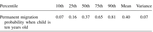
secondary track schools are decided, see Dustmann (2004) for details. We then nor-malize this variable between 0 and 1. We present the distribution of the resulting var-iable in Table 4. On average, the probability of remaining permanently in Germany for a father whose son is 10 years old is about 40 percent.
c. Selection issues
The sample of the foreign-born father-son pairs we use for analysis is one that is selected—we observe more father-son pairs where fathers have a higher propensity to stay permanently. This induces a selection, which is correlated with our measure for a permanent migration probability: Those with a higher probability of a permanent migration (measured by past intentions) will be more likely to be in the sample. If sons of those immigrants who remain in the sample perform differently than sons of those who return (conditional on father’s permanent earnings and per-manent migration probability), then this will bias the coefficient of the return prob-ability. The bias will be downward if residuals in the selection equation and the intergenerational mobility equation are positively correlated (indicating that sons of father-son pairs who remain in the sample do better than sons of father-son pairs who drop out of the sample, conditional on fatherÕs earnings and permanent migra-tion probability). The intuimigra-tion is that those who have a low probability to remain permanently, but are nevertheless in the sample, must have unobserved characteris-tics that are positively related to the son’s performance, which leads to a reduction of the coefficient estimate on the permanent migration probability in absolute size.10 We can therefore interpret the coefficients on the permanent migration measure as a lower bound.
Table 4
Distribution of Permanent Migration Probabilities
Percentile 10th 25th 50th 75th 90th Mean Variance
Permanent migration probability when child is ten years old
0.07 0.16 0.37 0.65 0.81 0.40 0.07
Source: GSOEP, various years.
10. More formally, suppose that the latent index for being selected into the sample, s*is linear in p, the probability of a permanent migration, withs
i¼a0+api+ui;and that a father-son pair is in the sample
ifs
i.0. Suppose that the outcome equation is given byyi¼g0+gpi+vi;and assume thatuiandviare
jointly normally distributed, with variances 1 andr2
vand correlation coefficientr. Then selection could
be accounted for adding the generalized residualEðvijsi.0Þ ¼lðciÞto the estimation equation, where lci¼fðciÞ=FðciÞ;withf andFbeing the density and distribution function of the standard normal,
andci¼a0+api. We obtain the estimation equationyi¼g0+gpi+rvplðciÞ+ei. Omission oflðciÞresults
IV. Results
B. Investment in Education
We commence by estimating investment equations. Our theoretical model relates in-vestment in children to fathersÔpermanent earnings, as well as to the probability of a permanent migration. As a measure for investment, we use the sonÕs educational out-comes. We concentrate here on secondary school track choice. Results on completed education are very similar, and we briefly discuss them.
In Germany, age 10 marks an important decision in the school career of children. At this age, the child transfers from primary to secondary school, and, at the same time, has to decide between three secondary school tracks: lower secondary (with graduation typically at age 16), intermediate secondary (with graduation typically at age 16–17), and upper secondary (with graduation typically at age 18–19). Al-though switching tracks is possible, it rarely occurs (see Pischke 1999 for evidence). Only high school allows for continuation to University; lower and intermediate secondary schools qualify for blue collar and white-collar apprenticeship degrees.11 Initial track choice is therefore very important for future career prospects. Dustmann (2004) illustrates the strong correlation between secondary school track, post-secondary educational achievements, and earnings.12
The main objective of our analysis is to understand the relationship between the probability the father assigns to a permanent migration and the educational qualifi-cations of the son. We also investigate the relationship between the father’s perma-nent earnings and school track enrollment of the son. And finally, we investigate the possible correlation between the childÕs educational achievements and education of the father, and compare this for immigrants and natives.
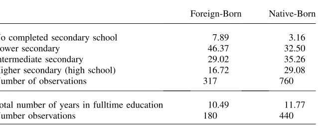
In Table 5, we display secondary school degrees for sons of native- and foreign-born fathers. The numbers show that sons of native-born fathers have a higher probability of attending higher track schools than the sons of foreign-born fathers. While about 64 percent of sons of native-born fathers attend at least an intermediate secondary school, this number is only 46 percent for sons of foreign-born fathers. On the other hand, about 8 percent of sons of foreign-born fathers do not complete secondary school training, while this is the case for only 3 percent of sons of native-born fathers.
The numbers in the lower panel give the total number of years of education for the two groups. There is a difference in the number of years of full-time education be-tween sons of native- and foreign-born fathers of about 1.3 years, which is a signif-icant reduction compared to the fathers’ generation, where this difference was 2.4 years (see Table 2).
Our sample includes all sons above the age of 15, even if they are still in secondary education, because the secondary school choice has been made before that age. We
also report results for completed education, measured as the total number of years in full-time education for those who have finished full-time education.
In Table 6, we present results from an ordered probit model of secondary school choice. We report results for sons of foreign-born fathers (upper panel), and of native-born fathers (lower panel). As in Table 5, we distinguish between four levels: no completed secondary school, lower secondary school, intermediate secondary school, and high school.13In all regressions we condition on the son’s birth cohort, the age of the father when the son was 10-years-old, and (for foreign-born fathers) on the country of fatherÕs birth (coefficients are not reported).
In the left panel, we present estimation results of coefficients on the father’s per-manent migration probability only (Column 1), and when we condition in addition on the fatherÕs permanent log wage (where we use estimates based on a minimum of five wage spells), and his years of education (Columns 2). In Appendix Table A3, we report the marginal effects of these variables on the probability that the son does not obtain a secondary school degree (first column), and achieves a high school degree (second column). These probabilities are calculated at sample means for each sample.
The coefficient on the measure of a permanent migration probability is significantly different from zero (Table 6, Column 1). Unconditional on the father’s permanent earnings and education, an increase in the probability of remaining permanently of one standard deviation is associated with an increase in the probability of high school attendance of about four percentage points. Given that only about 17 percent of sons Table 5
Educational Attainments, Sons of Foreign- and Native-Born Fathers
Foreign-Born Native-Born
No completed secondary school 7.89 3.16
Lower secondary 46.37 32.50
Intermediate secondary 29.02 35.26
Higher secondary (high school) 16.72 29.08
Number of observations 317 760
Total number of years in fulltime education 10.49 11.77
Number observations 180 440
Source: GSOEP, various years.
Note: sample for track choice includes all sons above the age of 15, even if they are still in secondary ed-ucation, as the secondary school choice has been made before that age. Fulltime education is measured as the total number of years in fulltime education for those who have finished fulltime education.
13. The underlying latent model for school track choice is given byEdi¼x 0
ib+aEdfi+gPi+ui;whereEdiis
an index for track choice of individual i,Edfiis the level of education ofi’s father (measured in years),Pithe
father’s return probability, andxia vector of characteristics, including son’s cohort and father’s country of
or-igin and age, and whereui;Nð0;r2Þ:The observed variableEd
iis related to the latent index as follows:
Edi¼kiffEdsi2 ðuk21;uk;wherek¼1,2,3,4. Hereu0¼2Nandu4¼N. The realizationsEdi¼k
Table 6
Educational Investment
1 2 3 4
Secondary school track choice Coefficient
Standard
Error Coefficient
Standard
Error Coefficient
Standard
Error Coefficient
Standard Error
Foreign-born fathers
Probability of permanent migration 0.612 0.262 0.571 0.315
Father’s permanent log wage 0.804 0.410 0. 879 0.349
Father’s years of education 0.040 0.037 0.057 0.034
Number of observations 314 309 307 551
Native-born fathers
Father’s permanent log wage 1.106 0.127
Father’s years of education 0.219 0.023
Number of observations - - 620 757
Source: GSOEP, various years.
Note: Ordered probit estimates, dependent variable: secondary school track. All estimation equations include son’s birth cohort, the age of the father when the son is 10 years old, and (for the foreign-born) father’s country of origin dummies.
The
Journal
of
Human
of foreign-born parents attend high school, this impact is quite large. In Column 2, we condition in addition on the fatherÕs permanent wages and on the father’s years of education. This specification corresponds to the investment equation in Equation 4. Conditioning on the fatherÕs schooling should further eliminate influences that affect both the son’s educational attainment, and remigration probabilities. The size of the coefficient of the permanent migration probability reduces only slightly if we condi-tion on these variables. Thus, condicondi-tional on the fatherÕs level of education, age, and permanent wages, a sizable difference remains in enrollment in higher track schools between those whose fathers tend to remain permanently in the host country, and those whose fathers do not. The coefficient estimate on the father’s permanent wage is positive and significant. An increase in fatherÕs permanent log wage by one standard deviation (0.21) increases the probability that the son will enroll in a higher secondary school by about four percentage points (see Appendix Table A3).
In Columns 3 and 4, we report results for estimation equations conditioning only on permanent log wages, and on fathersÔeducation, for both foreign (upper panel) and native-born (lower panel) father-son pairs. The latter equation is frequently es-timated in the literature on the intergenerational mobility of education. Within our investment model, it can be interpreted as a reduced-form equation, where the effect of fathersÕeducation on sonsÔeducational attainments works through fathersÕ perma-nent wages. For foreign-born fathers, the father’s years of education is insignificant, but it is highly significant (and much larger) for native-born fathers. For the latter group, each year of additional education increases the probability that the son attends high school by 7.3 percentage points. These results support estimates by Gang and Zimmermann (2000), who do not find any association in education between for-eign-born parents and their children. This may be, in their case, because their sample includes immigrants who arrived before the age of 16, and have therefore obtained or started education in their home countries. In our case, all sons of foreign-born parents are born in Germany; despite that, we find only small and insignificant associations between fathers and sonsÕeducational attainments.
We have also estimated the same specifications for the completed number of years of education for those sons who completed full-time education on father’s permanent migration probabilities (results not reported). Estimation results are very similar. As for the track choice, sons of fathers who have a higher probability of remaining per-manently have significantly higher completed levels of education. Conditioning on the fatherÕs permanent log wage and level of education in addition, reduced the co-efficient estimate only slightly, and is largely in line with track choice results reported above. When we estimate investment equations conditioning only on the father’s permanent wage or the fatherÕs years of education in addition, the coefficient on the father’s permanent earnings is remarkably similar for natives and immigrants, suggesting that an increase in permanent wages of 10 percent increases years of ed-ucation by about 0.18. As before, while for native fathers, eded-ucation is strongly and significantly associated with sonsÕeducation, it is smaller and insignificant for immi-grants.
Table 7
Intergenerational Correlation Coefficients, Foreign and Native Born Fathers
All More than 4 valid wage spells More than 7 valid wage spells
Coefficient
Standard
Error Coefficient
Standard
Error Coefficient
Standard Error
Foreign-born fathers 0.145 0.070 0.365 0.108 0.408 0.144
Number of observations 583 503 404
Number of groups 155 129 107
Native-born fathers 0.177 0.055 0.251 0.061 0.290 0.066
Number of observations 1,737 1,474 1,329
Number of groups 360 320 284
Source: GSOEP, various years.
Note: dependent variable: Son’s log hourly wage. Regression includes son’s age and age2, a linear time trend, and father’s country of origin dummies for individuals with a foreign-born father.
The
Journal
of
Human
estimates; however, it is unlikely to explain fully the large difference in point esti-mates for foreign- and native-born father-son pairs.14
A further explanation is that it is permanent earnings rather than educational achievements of the father that drives educational outcomes of the son. This interpre-tation is compatible with an intergenerational permanent income model, as the one we develop above. The association between fathers’ permanent earnings and sonsÕ
education that we estimate is similar for school track choice of foreign- and na-tive-born (Table 6), and near identical for completed full-time education. If education of the father affects the son’s education mainly through the fatherÕs earnings, a low correlation between permanent earnings and education—as often found in immigrant communities—explains why some studies (like Gang and Zimmermann 2000) find only a modest association of educational achievements between parent and offspring in immigrant samples.15
1. Intergenerational earnings correlation
a. Comparing Foreign- and Native-born Father-Son Pairs
We now turn to analysis of intergenerational mobility in permanent earnings, and on the impact of a permanent migration probability on permanent wages. In Table 7, we first report intergenerational correlation coefficients for both immigrants and natives, using the measure for fathers’ permanent log wage as de-scribed above. We ignore here the permanent migration variable for immigrants, but we use measures for fathersÕpermanent income that gradually remove measure-ment error. We use all wage information for sons, and report standard errors that al-low for an equi-correlated covariance matrix. Estimates are based on Equation 9, but include in addition a quadratic in son’s age and a linear time trend. The upper panel of Table 7 reports results for foreign-born fathers, and the lower panel reports results for native-born fathers.
The results in the first column are based on all available observations for construct-ing fathers’ log wages. Intergenerational correlation coefficients for natives as well as immigrants are small, and similar in magnitude to those reported by Crouch and Dunn (1997). In the second column, we use as a measure for parental permanent earnings predictions based on at least five wages spells. This should reduce any downward bias through measurement error. The effect on estimates is quite dramatic, with coefficients increasing to 0.25 for natives, and 0.36 for immigrants. The last col-umn reports estimates where only father-son pairs with fathers reporting at least eight wage spells are included. Coefficients rise further, to 0.29 for natives, and 0.40 for immigrants. Restricting the samples even further (we experimented with at least 11 wage observations for fathers) does not lead to any significant further change in the coefficients.
14. Assuming that measurement error is well-behaved, and taking the point estimates in the completed ed-ucation regressions at face value, the variance of the measurement error will need to be four times as large as the variance in fathers’ education to explain the difference in estimates between regression results for sons of foreign and native born fathers.
Table 8
Son’s Log Wages and Permanent Migration Probabilities, Foreign-Born Fathers
All
More than 4 valid wage spells
More than 7 valid wage spells
1 2 3 4
Coefficient
Standard
Error Coefficient
Standard
Error Coefficient
Standard
Error Coefficient
Standard Error
Father’s log wage — — 0.140 0.070 0.344 0.111 0.387 0.152
Father’s permanent migration propensity 0.186 0.081 0.197 0.083 0.130 0.090 0.110 0.103
Number of observations 591 568 488 389
Number of groups 159 153 127 105
Permanent migration probability based on information before son was 16 years old
Father’s log wage — — 0.289 0.104 0.322 0.149 0.364 0.181
Father’s permanent migration propensity 0.235 0.087 0.244 0.085 0.238 0.090 0.242 0.104
Number of observations 375 363 300 264
Number of groups 109 105 89 78
Source: GSOEP, various years.
Note: dependent variable: son’s log hourly wage. Regression includes son’s age and age2, a linear time trend, and father’s country of origin dummies.
The
Journal
of
Human
The increase in estimated coefficients is in line with other studies, suggesting substan-tial underestimation in the degree of intergenerational immobility through measurement error in parental earnings. The numbers further suggest a larger intergenerational immo-bility for immigrant father-son pairs than for native father-son pairs. The difference in point estimates, based on estimates in Column 3, is about 0.12; however, the difference is not significantly different from zero, which is perhaps not surprising given the small sam-ple size. The magnitude of estimates for immigrants is similar to that reported for the United States by Solon (1992) and Zimmermann (1992), who obtain coefficients of about 0.4. They also use multiyear averages to reduce measurement error in parental earnings. Our point estimates for natives are smaller than those in the U.S. studies. Bjørklund and Jantti (1997), using a method for estimating intergenerational income correlation on independent samples for Sweden, also conclude that Swedish estimates are smaller than those obtained for the United States.
b. Permanent Migration Probabilities
In Table 8, we report estimates for immigrants where we condition additionally on the father’s probability of a permanent migration, as suggested by Equation 9. Other regressors include, as before, a quadratic in the sonÕs age, the father’s origin dum-mies, and a time trend. The estimated coefficient of the measure for a permanent mi-gration suggests a higher log wage for sons whose fathers tend to consider the migration as permanent rather than temporary. The effect is sizable: An increase in the probability of a permanent migration by one standard deviation (0.26) increases the sonÕs permanent real wages by about 5 percent.
In the next columns, we condition in addition on the father’s permanent wages. Column 2 consider all father-son pairs with at least one observation on fathersÕ earn-ings, and Columns 3 and 4 restrict the sample to father-son pairs with more than four or seven earnings observations for the father. In Column 2, the coefficient on the father’s probability of a permanent migration remains roughly the same as in Column 1, with about the same standard error. Conditional on fathersÕpermanent earnings, an increase in the probability of the father staying permanently continues to increase the son’s permanent wage.
When using measures for fathers’ earnings that are based on more than four or seven wage observations (Columns 3 and 4), the coefficient on the measure for a per-manent migration propensity decreases in size, and is less precisely estimated. One reason for this is the reduction in sample size when we move to fathers with more than four, or seven valid wage spells. The decrease in the coefficient on the perma-nent migration probability could be due to the fatherÕs permanent earnings being pos-itively correlated with the father’s probability to migrate permanently. Therefore, a downward bias in the effect of fathersÕpermanent earnings on the son’s wage trans-lates into an upward bias in the coefficient estimate of the permanent migration prob-ability. Overall, return probabilities seem to be related to sonsÕpermanent earnings in a way that is compatible with the model, although the last estimates are not signif-icant.
c. Robustness checks
1. Simultaneity
One concern with our estimates is that fathers condition their own migration plans on the son’s labor market performance, which may lead to simulta-neity bias if we use information on the fatherÕs remigration plans after the son has entered the labor market. To check this, we have reestimated regressions in Table 8 using permanent migration probabilities that are constructed from the father’s responses before the son was 16 years old (which is the minimum age for labor mar-ket entry).
We present results in the lower panel of Table 8. The estimates for the permanent migration probability increase slightly in size, and remain stable and significant throughout the four specifications. Estimates for the three measures of the father’s permanent earnings are more similar in size across specifications than before. The reason is that the sample, which is based on permanent migration intentions before sons were 16 years old, excludes many of those fathers who have only a small num-ber of wage observations, thus reducing the measurement error bias from the start. Results confirm that there is a positive relationship between the fatherÕs permanent migration propensity and the child’s earnings along the lines we have hypothesized above.
Parents may have knowledge about their child’s future earnings performance be-fore their childÕs entry into the labor market, and condition their return intentions on this, which may then still lead to biased estimates. When using father-son pairs where migration probabilities are computed when the child was even younger leads to small samples. We have experimented with that, and used father-son pairs for which we can compute return probabilities for fathers based on survey information when the son was 13 years of age or younger. The sample size drops to 164 obser-vations when estimating specifications as in Column 3 of Table 8. The coefficient on the permanent migration probability is similar to that reported in Table 8: 0.266, with a standard error of 0.114.
2. Siblings
We include in our sample siblings who have the same father (see Table 1 for frequencies). To check if our results are robust to using only the oldest son for father-son pairs with more than one son, we reestimate the models restricting our sample to father-oldest son pairs if a father has more than one son. The results for the intergenerational correlation coefficients are similar, with point estimates and associated standard errors of 0.261 (0.058) and 0.278 (0.061) for natives, using wage information based on more than 5 or 7 years of the father’s wage data, and corresponding coefficients of 0.355 (0.165) and 0.360 (0.197) for immigrants. Point estimates remain higher for immigrant father-son pairs.
V. Discussion and Conclusions
Earlier research by Borjas (1992) suggests that the way wealth and earnings potential is transmitted from one generation to the next may differ between immigrant and native-born communities. Borjas argues that for immigrants the qual-ity of the ethnic environment may provide an externalqual-ity in the production of human capital of the next generation, which affects parental investments. In this paper we investigate a further reason why parental investment may be different across immi-grant groups: differences in parents’ assessment about a permanent or a temporary migration. We also estimate and compare intergenerational correlation coefficients for education and permanent earnings, distinguishing between immigrant and native-born father-son pairs. Our empirical analysis is based on a long panel that oversamples immigrants. The data provide unique and repeated information on per-manent migration intentions of foreign-born individuals.
To analyze parental investment in the son’s education, we investigate secondary school track choice. We find a strong association between the probability of fathersÕ
permanent migration, and sons’ educational attainments, conditional on the fatherÕs age and origin country, and the son’s cohort. These estimates remain similar if we condition in addition on fathersÕeducation, and on fathers’ permanent earnings.
For both native- and foreign-born fathers, the father’s permanent earnings posi-tively affect educational achievements of the son. For father-son pairs with native-born fathers, we also find a strong correlation between educational attainment of father and son, while this correlation is small and insignificant for immigrants. We explain this with the low association between education and earnings for foreign-born fathers: If parental earnings affect investment in the childÕs education, as sug-gested by the permanent income model of intergenerational mobility, then the father’s education is a weaker proxy for permanent earnings for immigrants than for natives.
Estimating intergenerational correlation coefficients in permanent earnings for father-son pairs of foreign- and native-born fathers, and taking account of measure-ment error using a flexible averaging method, we find intergenerational correlation coefficients of about 0.3 for father-son pairs with native-born fathers, and about 0.4 for father-son pairs with foreign-born fathers. Consistent with our hypothesis, we find for foreign-born fathers that the son’s permanent wages are positively asso-ciated with the probability of the fatherÕs permanent migration.
Frequencies of Earning Spells, Fathers
Years Foreign-Born Fathers Native-Born Fathers
Observed
earnings Individuals
Sum Percent
Sum Valid Spells
Sum Percent
Spells Individuals
Sum Percent
Sum Valid Spells
Sum Percent Spells
0 7 2.79 — — 23 3.59 — —
1 8 5.98 8 0.31 23 7.19 23 0.31
2 7 8.76 22 0.85 17 9.84 57 0.78
3 13 13.94 61 2.36 23 13.44 126 1.73
4 6 16.33 85 3.29 32 18.44 254 3.49
5 13 21.51 150 5.82 28 22.81 394 5.42
6 11 25.90 216 8.38 23 26.41 532 7.32
7 20 33.86 356 13.81 18 29.22 658 9.06
8 6 36.25 404 15.67 29 33.75 890 12.25
9 15 42.23 539 20.91 31 38.59 1,169 16.09
10 23 51.39 769 29.84 24 42.34 1,409 19.40
11 19 58.96 978 37.95 25 46.25 1,684 23.18
12 18 66.14 1,194 46.33 29 50.78 2,032 27.98
13 12 70.92 1,350 52.38 25 54.69 2,357 32.45
14 13 76.10 1,532 59.44 43 61.41 2,959 40.74
15 8 79.28 1,652 64.10 33 66.56 3,454 47.56
16 9 82.87 1,796 69.69 39 72.66 4,078 56.15
17 10 86.85 1,966 76.29 35 78.13 4,673 64.34
18 16 93.23 2,254 87.46 71 89.22 5,951 81.94
19 17 100.00 2,577 100 69 100.00 7,262 100.00
Total 251 — 2,577 — 640 — 7,262 —
Source: GSOEP, various years.
The
Journal
of
Human
Years Sons of Foreign Born Fathers Sons of Native Born Fathers
Observed
earnings Individuals
Sum Percent
Sum Valid Spells
Sum Percent
Spells Individuals
Sum Percent
Sum Valid Spells
Sum Percent Spells
0 173 51.80 2 2 423 53.14 2 2
1 48 66.17 48 7.92 68 61.68 68 3.73
2 31 75.45 62 18.15 63 69.60 126 10.64
3 12 79.04 36 24.09 47 75.50 141 18.37
4 21 85.33 84 37.95 25 78.64 100 23.85
5 10 88.32 50 46.20 24 81.66 120 30.43
6 9 91.02 54 55.12 31 85.55 186 40.63
7 7 93.11 49 63.20 22 88.32 154 49.07
8 9 95.81 72 75.08 21 90.95 168 58.28
9 5 97.31 45 82.51 22 93.72 198 69.13
10 4 98.50 40 89.11 20 96.23 200 80.10
11 1 98.80 11 90.92 9 97.36 99 85.53
12 — — — — 11 98.74 132 92.76
13 2 99.40 26 95.21 8 99.75 104 98.46
14 1 99.70 14 97.52 2 100.00 28 100.00
15 1 100.00 15 100.00 — — — —
Total 334 — 606 — 796 — 1,824 —
Source: GSOEP, various years.
Dustmann
Table A3
Secondary School Track Choice, Marginal Effects
1 2 3 4
No secondary
school
Highest secondary
school
No secondary
school
Highest secondary
school
No secondary
school
Highest secondary
school
No secondary
school
Highest secondary
school
Foreign Born Fathers
Probability of permanent migration 20.085 0.153 20.070 0.140
Father’s permanent log wage 20.098 0.197 20.133 0.240
Father’s years of education 20.005 0.010 20.008 0.013
Native Born Fathers
Father’s permanent log wage 20.066 0.399
Father’s years of education 20.011 0.073
Source: GSOEP, various years.
Note: marginal effects, ordered probits. Specifications as in Table 6. Probabilities are calculated at sample means for each of the two samples.
The
Journal
of
Human
References
Bauer, Philip, and Regina T. Riphan. 2004. ‘‘Heterogeneity in the Intergenerational Transmission of Educational Attainment: Evidence from Switzerland on Natives and Second Generation Immigrants.’’ Basel: University of Basel. Unpublished.
Becker, Gary, and Nigel Tomes. 1979. ‘‘An Equilibrium Theory of the Distribution of Income and Intergenerational Mobility.’’Journal of Political Economy87(6):1153–89.
__________. 1986. ‘‘Human Capital and the Rise and Fall of Families.’’Journal of Labor Economics4(3): S1–S39.
Bjørklund, Anders, and Markus Jantti. 1997. ‘‘Intergenerational Income Mobility in Sweden Compared to the United States.’’American Economic Review87(5):1009–18.
Bjørklund, Anders, Mikael Lindahl, and Erik Plug. 2006. ‘‘The Origins of Intergenerational Associations: Lessons from Swedish Adoption Data.’’Quarterly Journal of Economics
121(3): 999–1028.
Bohning, W. Roger. 1987.Studies in International Migration.New York: St. Martin’s Press. Borjas, George J. 1985. ‘‘Assimilation, Changes in Cohort Quality, and the Earnings of
Immigrants.’’Journal of Labor Economics3(4):463–89.
__________. 1992. ‘‘Ethnic Capital and Intergenerational Mobility.’’Quarterly Journal of Economics107(1):123–50.
__________. 1993. ‘‘The Intergenerational Mobility of Immigrants.’’Journal of Labor Economics11(1):113–35.
__________. 1994. ‘‘Long-Run Convergence of Ethnic Skill Differentials: The Children and Grandchildren of the Great Migration.’’Industrial and Labor Relations Review47(4): 553–73.
__________. 1994b. ‘‘The Economics of Migration.’’Journal of Economic Literature
32(4):1667–1717.
__________. 1995. ‘‘Ethnicity, Neighborhood, and Human Capital Externalities.’’American Economic Review85(3):365–90.
Card, David, John DiNardo and Eugena Estes. 1998. ‘‘The More Things Change: Immigrants and the Children of Immigrants in the 1940s, the 1970s, and the 1990s.’’ NBER Working Paper 6519.
Carliner, Geoffrey. 1980. ‘‘Wages, Earnings and Hours of First, Second and Third Generation American Males.’’Economic Inquiry18(1):87–102.
Chiswick, Barry. 1977. ‘‘Sons of Immigrants: Are they at an Earnings Disadvantage?’’
American Economic Review67(1):376–80.
__________. 1978. ‘‘The Effect of Americanization on the Earnings of Foreign-born Men.’’
Journal of Political Economy86(5): 897–921.
Couch, Kenneth A., and Thomas A. Dunn. 1997. ‘‘Intergenerational Correlation in Labor Market Status: a Comparison of the United States and Germany.’’Journal of Human Resources32(1):210–32.
Cortes, Kalena E. 2004. ‘‘Are Refugees Different from Economic Immigrants? Some Empirical Evidence on the Heterogeneity of Immigrant Groups in the United States.’’
Review of Economic and Statistics86(2):465–80.
Dearden, Lorraine, Steve Machin, and Howard Reed. 1997. ‘‘Intergenerational Mobility in Britain.’’ The Economic Journal 107(440):47–66.
Dustmann, Christian. 1997. ‘‘Differences in the Labour Market Behaviour between Temporary and Permanent Migrant Women.’’Labour Economics4(1):29–46. __________. 1999. ‘‘Temporary Migration, Human Capital, and Language Fluency of
Migrants.’’Scandinavian Journal of Economics101(2):297–314.
__________. 2004. ‘‘Parental Background, Secondary School Track Choice, and Wages.’’
Galor, Oded, and Oded Stark. 1990. ‘‘Migrants Savings, the Probability of Return Migration, and Migrants Performance.’’International Economic Review31(2):463–67.
Gang, Ira N., and Klaus F. Zimmermann. 2000. ‘‘Is Child Like Parent? Educational Attainment and Ethnic Origin.’’Journal of Human Resources35(3):550–69.
Nielsen, Helena S., Michael Rosholm, Nina Smith, and Leif Husted. 2001. ‘‘Intergenerational Transmissions and the School-to-Work Transition of 2nd Generation Immigrants.’’ Working Paper 01-04, Aarhus: Centre for Labour Market and Social Research.
Pischke, Jo¨rn-Steffen. 1999. ‘‘Does Shorter Schooling Hurt Student Performance? Evidence from the German Short School Years.’’ Cambridge, Mass.: MIT. Unpublished.
Plug, Erik. 2004. ‘‘Estimating the Effect of Mother’s Schooling on Children’s Schooling Using a Sample of Adoptees.’’American Economic Review94(1):358–68.
Riphahn, Regina T. 2001. ‘‘Dissimilation? The Educational Attainment of Second Generation Immigrants.’’ CEPR Discussion Paper No. 2903.
Solon, Gary. 1989. ‘‘Biases in the Estimation of Intergenerational Earnings Correlations.’’
Review of Economics and Statistics71(1):172–74.
__________. 1992. ‘‘Intergenerational Income Mobility in the United States.’’American Economic Review82(3):393–408.
__________. 1999. ‘‘Intergenerational Mobility in the Labor Market.’’ InHandbook of Labor Economics, Vol. 3A, ed. Orley C. Ashenfelter and David Card, 1761–1800. Amsterdam: North-Holland.
__________. 2002. ‘‘Cross-Country Differences in Intergenerational Earnings Mobility.’’
Journal of Economic Perspectives16(3):59–66.
__________. 2004. ‘‘A Model of Intergenerational Mobility Variation over Time and Place.’’ InGenerational Income Mobility in North America and Europe, ed. Miles Corak, 38-47. Cambridge, England: Cambridge University Press.
Van Ours, Jan C., and Justus Veenman. 2003. ‘‘The Educational Attainment of Second Generation Immigrants in The Netherlands.’’Journal of Population Economics16(4):739– 53.
Wiegand, Johannes. 1997.Four Essays on Applied Welfare Measurement and Income Distribution Dynamics in Germany 1985–1995.PhD Dissertation. London: University College London.
Woessmann, Ludger, and Eric A. Hanushek. 2006. ‘‘Does Educational Tracking Affect Performance and Inequality? Differences-in-Differences Evidence across Countries.’’
Economic Journal116 (510): C63–C76.