The Effects of Minimum Wages on
the Distribution of Family Incomes
A Nonparametric Analysis
David Neumark
Mark Schweitzer
William Wascher
A B S T R A C T
An oft-stated goal of the minimum wage is to raise incomes of poor or low-income families. We present nonparametric estimates of the effects of mini-mum wages on the distribution of family income relative to needs in the United States. Although minimum wages increase the incomes of some poor families, the evidence indicates that their overall net effect is, if anything, to increase the proportions of families with incomes below or near the poverty line. It would appear that reductions in the proportions of families that are poor or near-poor should not be counted among the potential benefits of minimum wages.
I. Introduction
Debates over the merits of a higher minimum wage frequently focus on the potential for employment losses from a higher wage floor. However, the exis-tence of negative employment effects does not necessarily imply that minimum wages constitute bad social policy. Employment losses associated with a higher minimum wage may be acceptable if the increase in the minimum raises the incomes of poor or near-poor families. To quote Gramlich (1976): “Minimum wages do, of course, distort
David Neumark is Senior Fellow, Public Policy Institute of California, a Research Associate of the NBER, and a Research Fellow at IZA Research at UC-Berkeley. Mark Schweitzer is Assistant Vice President and Economist, the Federal Reserve Bank of Cleveland. William Wascher is Deputy Associate Director in the Division of Research and Statistics at the Board of Governors of the Federal Reserve System. The authors thank Rebecca Blank, Harry Holzer, Sanders Korenman, Thomas Lemieux, Walter Oi, Dan Sichel, anony-mous referees, and seminar participants at Essex University, Michigan State, NYU, Northwestern, Berkeley, UC-Irvine, VPI, and the OECD for helpful comments. The views expressed are those of the authors only, and do not necessarily reflect those of the Public Policy Institute of California, the Federal Reserve Board, the Federal Reserve Bank of Cleveland, or their staffs. The data used in this article can be obtained beginning May 2006 through April 2009 from Mark Schweitzer, Federal Reserve Bank of Cleveland, P.O. Box 6387, Cleveland, OH, 44101-1387, Mark.E.Schweitzer@clev.frb.org. [Submitted April 2002; accepted February 2004]
ISSN 022-166X E-ISSN 1548-8004 © 2005 by the Board of Regents of the University of Wisconsin System
relative prices, and hence compromise economic efficiency, but so do all other attempts to redistribute income through the tax-and-transfer system. The important question is not whether minimum wages distort, but whether the benefits of any income redistrib-ution they bring about are in some political sense sufficient to outweigh the efficiency costs” (p. 410). Our goal in this paper is to provide information that helps in assessing this tradeoff.
Two empirical questions underlie the redistributive effects of minimum wages. First, how do minimum wages affect the total earnings of the low-wage work force; that is, do the wage gains received by employed workers more than offset the earn-ings lost by those who lose or cannot find jobs?1Second, how do minimum wages impact workers in different parts of the family income distribution? Because not all minimum-wage workers are in poor families (Gramlich 1976; Card and Krueger 1995; Burkhauser, Couch, and Wittenburg 1996), the incidence of gains and losses to workers in different parts of the family income distribution will have an important influence on the effects of minimum wages on low-income families.
In this paper, we provide nonparametric density estimates of the effects of mini-mum wages on family incomes. Specifically, we use matched March CPS data on families to study how the distribution of family incomes relative to needs is affected by an increase in the minimum wage. In a nutshell, our empirical strategy is to com-pute difference-in-difference estimates of the effects of minimum wages on the fam-ily income-to-needs distribution, by comparing changes in this distribution over time in states in which minimum wages did and did not increase.
This approach has some important advantages relative to existing work on the effects of minimum wages on the income distribution. First, most of the well-known papers on this topic, including Gramlich (1976), Johnson and Browning (1983), Burkhauser and Finegan (1989), and Horrigan and Mincy (1993), do not directly esti-mate the consequences of minimum-wage increases for family incomes, but rather makes use of simulations that are based on assumptions about employment effects and other relevant parameters. In contrast, we conduct an actual “before and after” analy-sis of the effects of minimum wages on family incomes. Second, the few papers that do use actual changes in family income to infer the effects of minimum wages focus on a specific parametric question that is an isolated part of the whole picture. For exam-ple, Addison and Blackburn (1999) estimate the effects of minimum wages on state poverty rates for relatively narrow subsets of the population. Similarly, Card and Krueger (1995) estimate the effect of the minimum wage on state poverty rates and on weekly family earnings at a few specific centiles, Neumark and Wascher (2002) focus on transitions in and out of poverty, and Connolly and Segal (1997) estimate average earnings changes experienced by families in different ranges of income-to-needs.2
1. In contrast, DiNardo, Fortin, and Lemieux (1996) focus on the effects of minimum wages on the distri-bution of wages of employed workers.
In contrast, our nonparametric approach provides a full picture (literally) of the effects of minimum wages on the shape of the family income distribution and on changes in incomes of families at different points in the income distribution. For example, we can examine the extent to which minimum wages push families initially near-poor into poverty, or lift initially poor families out of poverty. Importantly, the nonparametric approach provides a far richer empirical description of the effects of minimum wages on family incomes than would a regression-based approach that arbi-trarily specifies particular points of the distribution and asks whether the proportions of families above or below those points increase or decrease. On the other hand, as we explain in detail in Section III, the nonparametric estimation comes at some cost, most notably the added complexities of recovering estimates of the combined effects of contemporaneous and lagged increases in minimum wages, and the inability to fully exploit continuous variation in the minimum wage. In our view, the advantages of the nonparametric approach outweigh the disadvantages. Regardless, it clearly provides complementary evidence to parametric approaches.
The evidence on both the distributions of family income and of changes in incomes experienced by families in different parts of the distribution indicates that raising the minimum wage tends, if anything, to increase the proportions of families that are poor or near-poor and to reduce the proportion of families with incomes above the “near-poverty” line but below about three times the poverty line. This evidence implies that reductions in the proportions of families that are poor or near-poor should not be counted among the potential benefits of minimum wages.
II. The Data
The data we use come primarily from matched March CPS annual demographic files from 1986 through 1995. Using matched data from the CPS pro-vides an important advantage relative to an analysis of the annual CPS cross-sections. In particular, the availability of two consecutive years of data for each family allows us to observe their transitions between various parts of the income distribution. As a result, when we observe a change in the income-to-needs distribution, we can more comfortably conclude that this change reflects the actual experiences of families rather than differences in the set of families sampled in each year. Statistically, the homogeneity of the samples before and after the minimum-wage increase leads to more precise inferences.
Our choice of sample period was influenced by three factors. First, our ability to match successive March files for consecutive years is limited to this ten-year time period. In particular, it is not possible to match CPS files from 1985 with those in 1986 because the two files are based on different Census sample designs; for similar reasons, it is also not possible to match the 1995 files with those in 1996. Second, for reasons discussed below, it is desirable to use a sample period with considerable state variation in minimum wages, and it was in the late 1980s that such variation first emerged. Third, changes in state welfare rules associated with the 1996 welfare reform legislation would confound estimation of minimum-wage effects if, as seems likely, these changes altered the labor market behavior of low-income families. By ending the sample in 1995 and focusing on the prereform period, we avoid this
tial bias, although we obviously cannot decisively rule out contaminating influences of other state-level policy changes.3
For each family, we extracted information on family income, family size, and the family’s state of residence.4We take a reduced form approach that does not distin-guish among families based, for example, on whether family size changed, someone retired, or there was any earned income. Instead, we treat the family as the unit of observation and infer the total effect of minimum-wage changes through any of these channels. However, the type of analysis we carry out here can be extended to study the mechanisms by which family incomes (relative to needs) are affected.
In all cases, the income data refer to the previous calendar year; although the state of residence is contemporaneous, the matching process ensures that only families liv-ing at the same address in two consecutive years are included in the data. We follow other research in this area in looking at total family income from all sources. Given the family income data, each family is classified in terms of its income-to-needs ratio (the ratio of total family income to the poverty line for that family). The estimation is conducted for families with nonnegative incomes, up to a maximum income-to-needs ratio of six.
Each family-year record is also assigned the minimum-wage level that prevailed in the state in May of the year for which family income is measured, as well as the min-imum wage in the preceding year.5Because state minimum-wage laws do not exempt employers of workers covered by the federal law from the federal minimum wage, and because coverage by the federal law is nearly complete, we use the higher of the federal minimum wage and the state minimum wage for each state and year.
Table 1 reports the effective minimum-wage rates for each state over our sample period. The first column reports the minimum wage prevailing in 1987, while the remaining columns report the new minimum wage following an increase. With the exception of Minnesota, Pennsylvania, and New Jersey, all of the state increases occurred in the New England and Pacific states. Also noteworthy, however, is that a high fraction of the minimum-wage increases in this sample period stemmed from changes in the federal law. Because increases in the federal minimum have often coin-cided with sharp increases in overall unemployment rates (for example, in 1991), we cannot treat minimum wages as randomly assigned, but instead must attempt to account for the relationship between minimum wages and the business cycle to draw causal inferences regarding the effects of minimum wages on family incomes.
We also extracted the family-specific sampling weight, which we then adjusted to account for the possibility that certain types of families have a lower probability of being in the survey in consecutive years and thus are less likely to be included in our matched sample. In particular, although overall match rates were above 80 percent, families with younger heads and lower income-to-needs ratios were significantly less
3. On the other hand, a potential limitation of this data restriction is that minimum-wage effects could dif-fer in the environment created following welfare reform.
4. We use the CPS definition of a family, which is a group of two or more persons (one of whom is the householder) residing together and related by birth, marriage, or adoption. All persons satisfying these cri-teria, including related subfamily members, are considered members of one family.
Neumark, Schweitzer
, and W
ascher
871
Table 1
Minimum Wages by State and Year
1987 1988 1989 1990 1991 1992 1993 1994 1995
ME 3.65 — 3.75 3.85 4.25 — — — —
NH 3.45 3.55 3.65 3.80 4.25 — — — —
VT 3.45 3.55 3.65 3.85 4.25 — — — 4.50
MA 3.55 3.65 3.75 3.80 4.25 — — — —
RI 3.55 3.65 4.00 4.25 4.45 — — — —
CT 3.37 3.75 4.25 — 4.27 — — — —
NY 3.35 — — 3.80 4.25 — — — —
NJ 3.35 — — 3.80 4.25 5.05 — — —
PA 3.35 — 3.70 3.80 4.25 — — — —
OH 3.35 — — 3.80 4.25 — — — —
IN 3.35 — — 3.80 4.25 — — — —
IL 3.35 — — 3.80 4.25 — — — —
MI 3.35 — — 3.80 4.25 — — — —
WI 3.35 — — 3.80 4.25 — — — —
MN 3.35 3.55 3.85 3.95 4.25 — — — —
IA 3.35 — — 3.85 4.25 4.65 — — —
MO 3.35 — — 3.80 4.25 — — — —
ND 3.35 — — 3.80 4.25 — — — —
SD 3.35 — — 3.80 4.25 — — — —
NE 3.35 — — 3.80 4.25 — — — —
KS 3.35 — — 3.80 4.25 — — — —
DE 3.35 — — 3.80 4.25 — — — —
MD 3.35 — — 3.80 4.25 — — — —
VA 3.35 — — 3.80 4.25 — — — —
WV 3.35 — — 3.80 4.25 — — — —
NC 3.35 — — 3.80 4.25 — — — —
The Journal of Human Resources Table 1 (continued)
1987 1988 1989 1990 1991 1992 1993 1994 1995
SC 3.35 — — 3.80 4.25 — — — —
GA 3.35 — — 3.80 4.25 — — — —
FL 3.35 — — 3.80 4.25 — — — —
KY 3.35 — — 3.80 4.25 — — — —
TN 3.35 — — 3.80 4.25 — — — —
AL 3.35 — — 3.80 4.25 — — — —
MS 3.35 — — 3.80 4.25 — — — —
AR 3.35 — — 3.80 4.25 — — — —
LA 3.35 — — 3.80 4.25 — — — —
OK 3.35 — — 3.80 4.25 — — — —
TX 3.35 — — 3.80 4.25 — — — —
MT 3.35 — — 3.80 4.25 — — — —
ID 3.35 — — 3.80 4.25 — — — —
WY 3.35 — — 3.80 4.25 — — — —
CO 3.35 — — 3.80 4.25 — — — —
NM 3.35 — — 3.80 4.25 — — — —
AZ 3.35 — — 3.80 4.25 — — — —
UT 3.35 — — 3.80 4.25 — — — —
NV 3.35 — — 3.80 4.25 — — — —
WA 3.35 — 3.85 4.25 — — — 4.90 —
OR 3.35 — — 4.25 4.75 — — — —
CA 3.35 — 4.25 — — — — — —
AK 3.85 — — 4.30 4.75 — — — —
HI 3.35 3.85 — — 4.25 4.75 5.25 — —
likely to be successfully matched. Using a logistic regression that included the age and race of the family head and the income-to-needs ratio as categorical variables, we estimated the probability of a successful match for each family, and divided the sam-pling weight for successfully matched families by this estimated match rate. The adjusted weight is an estimate of the inverse of the probability of being in our matched sample of families.
III. Empirical Methods
A. Basic Strategy
In this section, we describe our strategy for estimating the effects of minimum-wage increases on the distribution of family income-to-needs. Our basic approach is to con-struct a difference-in-difference estimator. The treatment group is defined as the set of families residing in states in which the minimum wage rose between Years 1 and 2; the control group thus consists of families in states in which the minimum wage remained constant between Years 1 and 2. Letting numbers in the subscripts denote years, and MW = 1 and MW = 0 denote the treatment and control groups, we use f1,MW=1(I) to denote the density of income-to-needs in Year 1 in the treatment group and f2,MW = 1(I) to denote the density in Year 2 in the treatment group. The difference f2,MW = 1(I) − f1,MW = 1(I) measures the change in the density at each point Ifor this group. Because the density of income-to-needs may be changing for reasons other than minimum-wage increases, we subtract off the corresponding quantity for the control group, f2,MW = 0(I)
−f1,MW = 0(I). This yields the difference-in-difference estimator of the effect of mini-mum-wage increases on the density at each income-to-needs ratio I:
(1) {f2,MW = 1(I) −f1,MW = 1(I)} −{f2,MW = 0(I) −f1,MW = 0(I)}.
Although this approach does not provide explicit estimates of the influences of various regression controls, it potentially accounts for a wide range of factors that might alter the distribution of income. For example, business cycles and the corre-sponding changes in unemployment rates, rising earnings inequality stemming from other sources, and demographic trends (all national phenomena) are controlled for if these effects are equally evident in the treatment and control groups; below, we ask whether this condition is likely to hold, and explain how we account for such factors if it does not. In addition, an advantage of the nonparametric approach is that, unlike in a regression framework, the effectiveness of these controls does not rely on the linearity of any relationship with respect to the distribution of family income to needs.
To estimate each of the four densities in this expression, we use a kernel estimator. In particular, given a kernel K(z), the estimated density function for Iis:
(2) f I
n h K h
I I 1
k
e j j
j n
1
=
-i
=
!
^ h > H,
where nis the number of observations in the sample, his the bandwidth, and θjis a
sampling weight that has been normalized to sum to 1. The points at which the den-sity is estimated are indicated by I, and the data by Ij. The initial bandwidth is chosen
according to a normal rule of thumb procedure. Under this rule of thumb, the band-width used is optimal (in a RMSE sense) if the data are generated from a normal dis-tribution. In segments of the distribution with fewer observations, the bandwidths are adjusted to be wider using the adaptive bandwidth rule of Silverman (1986). In con-trast, the bandwidths are adjusted to be narrower in ranges where there are many observations to allow for sharper fluctuations in the estimated density in those ranges (Härdle 1991). Because the peak of the family income-to-needs distribution is typi-cally near one (the poverty line), this technique increases the accuracy of the kernel procedure in the area that may be of greatest interest.
We also apply these methods to analyze the densities of changes in to-needs, in which case we study subsamples of observations based on Year 1 income-to-needs. To accommodate the widely differing sample sizes that result from this disaggregation, we pool the data for initial bandwidth selection following Marron and Schmitz’s (1992) approach. This keeps the level of smoothing equal for the analyses of families in different initial income-to-needs categories, whereas standard rules would result in more smoothed estimates for smaller sample sizes.
B. Contaminated Treatment and Control Groups
Because previous research has found that the effects of minimum wages are often stronger at a lag of one year (see Neumark and Wascher 1992 and 2002, and Baker, Benjamin, and Stanger 1999), we are interested in estimating both contemporaneous and lagged minimum-wage effects on the densities of family income-to-needs. However, introducing lagged effects into our analysis creates complications because the observations for the treatment group (or the control group) may be contaminated by the effects of minimum-wage increases not directly captured by the difference-in-difference estimator. For example, when we estimate f2,MW = 1(I) for the treatment group for the lagged effect, there could also be a contemporaneous effect in Year 2. Similarly, when we estimate the density for the treatment group for the contempora-neous effect, there could be a lagged effect (from a contemporacontempora-neous increase in Year 1). Of course, we could drop all of the observations in which the treatment is con-taminated. But as Table 1 shows, that would entail the loss of many observations.
Instead, we employ a procedure that uses all of the observations and distributes the overall effects into “pure” contemporaneous and “pure” lagged effects correcting for the incidence of contaminated treatment and control groups. This procedure, which is explained in Appendix 1, turns out to have only a modest effect on the estimates.
C. Controlling for Other Differences Between Treatment and Control Groups
differences in movements of families through the income-to-needs distribution, per-haps also stemming from policy differences.
We first take a crude approach to eliminating the spurious influence of the business cycle on the estimates. In particular, the years in our sample in which the federal mini-mum wage was raised coincided with the recession in the early 1990s and thus with rel-atively sharp increases in state unemployment rates. As it seems unlikely that the federal minimum-wage increases actually caused the recession, we also present estimates in which we exclude the years influenced by a federal minimum-wage increase (1990 and 1991 as well as 1992, in which the lagged increase from 1991 occurred). This restric-tion avoids confounding the influence of the recession with minimum-wage effects, although it also likely goes too far in eliminating useful variation in the data.
An alternative and more informative approach is to mimic a regression model that includes fixed year and state effects. To do this, we first estimate the median propor-tional change in income-to-needs by state (across all years). We then adjust each fam-ily’s income-to-needs in Year 2 so that this common state change is taken out of the change in the family’s income-to-needs from Year 1 to Year 2. We make a parallel adjustment for the median proportional change by year (across all states).6The dif-ference between the adjusted data on income-to-needs for each family in Year 2 and Year 1 is the deviation around the average state change over all years in the sample and the average year change over all states in the sample. We then perform the basic difference-in-difference analysis described above using these adjusted data.
D. State versus Federal Increases and Biases from Migration
A third potential bias in our estimates relates to the possibility of migration. Because we rely partly on state minimum-wage increases to identify the effects of minimum wages and because changes in state minimum wages may influence the decision by workers and firms to move into or out of a state, the effects identified from state min-imum-wage increases may differ from the effects of federal increases. As an example, Cushing (2003) finds that poor families tend to migrate into a state in response to min-imum-wage increases. The magnitude of the migration response is modest, especially relative to the nonmigratory population, suggesting that it probably has only a small impact on our estimates. Moreover, any effect will be muted considerably in our data because migrants are not in the matched CPS data; thus, we would only detect the indirect effects of migration on those who already resided in the state.
Nonetheless, the presence of migration will lead our estimates to overstate the adverse impact of a federal minimum-wage increase (in response to which migration cannot really occur). In particular, if poor families migrate into a state that has
Neumark, Schweitzer, and Wascher 875
recently raised its minimum wage, then poor families already in the state may face slightly more labor market competition, while poor families remaining behind in other states may face slightly less, thereby worsening outcomes in the treatment group and improving them in the control group.7On the other hand, since the last federal minimum-wage increases in the mid-1990s, all of the changes in minimum wages in the United States have been at the state level. For these increases, our method likely understates (again, only slightly) the effects of the minimum wage because our sam-ple includes some federal variation.
IV. Results
A. Difference-in-Difference Estimates of Minimum-wage Effects on Income-to-Needs Densities
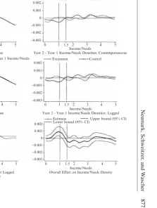
Figure 1 displays the entire set of density estimations that we use to infer the effects of minimum-wage increases on the distribution of income-to-needs. The first row presents evidence on changes in the income-to-needs distribution in states with con-temporaneous minimum-wage increases compared to states with no concon-temporaneous minimum-wage increases. The lefthand panel presents estimates of the densities in Year 1 and Year 2 for the treatment group (observations with increases), while the middle panel presents the corresponding densities for the control group. The vertical axis shows the proportion of families at each income-to-needs level. Because the dif-ferences between the densities in each panel are small relative to the scale (and there-fore hard to distinguish visually), the righthand panel summarizes the information by plotting—for the treatment and control groups, with a different scale—the vertical distance between the Year 1 and Year 2 densities.
The difference-in-difference estimate of the effects of contemporaneous minimum-wage increases on income-to-needs is the vertical distance between these two lines. Applying the methods described in the previous subsection (and in Appendix 1) yields the “pure” effect of a contemporaneous minimum-wage increase, which is displayed in the lefthand panel of the bottom row of Figure 1. Aside from the adjustment made to remove the influence of contaminated contemporaneous effects, this panel depicts the vertical distance between the solid and hatched graphs in the upper righthand panel.8 The results indicate that the effect of contemporaneous minimum-wage increases is to reduce the proportion of families with income-to-needs between 0 and about 0.6, to increase the proportion with income-to-needs between 0.6 and 1.5, and to reduce the proportion with income-to-needs from 1.5 to about 2.7. These results are consistent with minimum wages helping the poorest families, but they also suggest that families with initial income-to-needs in the range from 1.5 to about 2.7 experience income losses.
7. Migration in response to policy has received a fair amount of attention in the welfare literature. Recent work by Gelbach (2004) suggests that migration responses are real, but sufficiently small to have negligible consequences for estimation of other behavioral relationships.
Neumark, Schweitzer
, and W
ascher
877
Year 2 Income/Needs Year 2 Income/Needs
Year 2 Income/Needs
Year 1 Income/Needs Year 1 Income/Needs
Year 2 Income/Needs Year 1 Income/Needs
Treatment Control
Treatment − Control Densities for Contemporaneous
Minimum Wage Increase
Income/Needs No Minimum Wage Increase
Income/Needs
Year 2 - Year 1 Income/Needs Densities: Contemporaneous
Income/Needs
Year 2 - Year 1 Income/Needs Densities: Lagged Income/Needs
No Minimum Wage Increase
Income/Needs
Treatment − Control Densities for Lagged
Minimum Wage Increase
The panels in the second row of the figure report similar estimations, but with the treat-ment group defined as those observations for which there was a lagged minimum-wage increase. The righthand panel again shows the vertical distances between the Year 1 and Year 2 densities in the treatment and control groups. The difference-in-difference estimate of the pure lagged minimum-wage effect is reported in the middle panel of the bottom row. In contrast to the estimated effects of contemporaneous minimum-wage increases, lagged increases unambiguously raise the proportion of families below about 1.3 times the poverty line, with corresponding decreases in the proportion of families with income-to-needs between 1.3 and 3.2. This evidence, and the contrast with contemporaneous effects, is consistent with disemployment effects (or hours reductions) occurring with a lag.
The total effect of minimum-wage increases, shown in the bottom righthand panel, is the sum of the contemporaneous and lagged effects. The estimated effect at each particular point of the income-to-needs distribution is given by the middle curve, while the upper and lower curves are the tails of the 95 percent confidence interval, calculated using a bootstrap procedure for the nonparametric estimation.9The result is quite striking. There is essentially no net change in the proportion of families with income-to-needs below 0.3, as the benefit associated with the contemporaneous increase is offset by the cost of the lagged increase. There is a marked increase in the proportion of families with income-to-needs between about 0.3 and 1.4, and a marked decrease in the proportion of families with income-to-needs between about 1.4 and 3.3. These results suggest that the overall net effect of minimum-wage increases is to push some families that are initially low-income but above the near-poverty line into poverty or near-poverty. In addition, the estimated increases in the proportions of fam-ilies with income-to-needs from about 0.6 to 1.2 are statistically significant.
The first row of Table 2 provides some summary information about the changes in densities displayed in Figure 1. In particular, policymakers may be more interested in knowing, for example, whether minimum-wage increases lead to a statistically sig-nificant increase in the proportion of families below the poverty line than in the change in the proportion of families at a particular point of the income-to-needs dis-tribution. Thus, the table reports the estimated changes (and corresponding standard errors from the bootstrap) for some of the more “meaningful” ranges of income-to-needs. As indicated in Column 1, an increase in the minimum wage has essentially no effect on the proportion of families with income-to-needs between 0 and 0.5. In con-trast, as shown in Columns 2 and 3, minimum-wage hikes lead to an increase of 0.0079 in the proportion of families with income-to-needs between 0.5 and 1 and an increase of 0.0083 for the 0–1 category as a whole. The proportion of poor families in the sample is approximately 0.18, so that the change in the proportion poor corre-sponds to a 4.6 percent increase in the number of families with incomes below the poverty line. As indicated by the standard errors, the change in the proportion of fam-ilies between 0 and 0.5 is not statistically significant, while the changes in the pro-portion between 0.5 and 1 and the propro-portion below one are statistically significant.10
Neumark, Schweitzer
, and W
ascher
879
Table 2
Estimated Effects of Minimum Wage Increases on Proportions in Income-to-Needs Ranges
Income-to-Needs Categories
0–1, 1–1.5, 0–1.5, Poor/
0–.5 .5–1 In Poverty Near-Poor Near-Poor 1.5–2 2–3 1.5–3
Changes in proportions (1) (2) (3) (4) (5) (6) (7) (8)
No controls 0.0005 0.0079 0.0083 0.0046 0.0130 −0.0049 −0.0071 −0.0120
(0.0018) (0.0025) (0.0035) (0.0027) (0.0040) (0.0028) (0.0031) (0.0040)
No controls, exclude years 0.0055 0.0121 0.0176 0.0102 0.0278 −0.0028 −0.0300 −0.0328
with current or lagged (0.0040) (0.0058) (0.0086) (0.0065) (0.0108) (0.0071) (0.0088) (0.0114)
federal minimum wage increases (1990–1992)
Fixed state and year effects 0.0002 0.0069 0.0071 0.0033 0.0104 −0.0072 −0.0074 −0.0146
(proportional shifts) (0.0022) (0.0028) (0.0039) (0.0034) (0.0046) (0.0033) (0.0037) (0.0048)
N 9,030 15,738 18,954 18,725 36,525
As was apparent in Figure 1, Column 4 shows a sizable increase in the proportion of near-poor families (0.0046, or 3.6 percent) following minimum-wage changes, an estimate that is statistically significant at the 10 percent level. Column 5 aggregates over the preceding categories and shows that minimum-wage increases raise the pro-portion of poor or near-poor families by 0.013, an estimate that is again statistically significant. Columns 6-8 indicate that minimum-wage increases lead to declines in the proportion of families with income-to-needs in the 1.5–2 or 2–3 category of 0.0049 and 0.0071, respectively, while the overall decline in the proportion of families with income-to-needs between 1.5 and 3 is 0.012 (3.4 percent); the latter two estimates are statistically significant at the 5 percent level, and the first at the 10 percent level. To interpret the magnitudes in Table 2, the average minimum-wage increase in our sam-ple is 43 cents, or about 10 percent. Thus, the elasticity of changes in the proportion poor or near-poor with respect to the minimum wage is approximately 0.41, and the elasticity of the proportion with income-to-needs in the 1.5–3 range is about –0.34.11
B. Controlling for Other Influences on the Income-to-Needs Distribution
By comparing changes in the income-to-needs density between those state/year pairs with minimum-wage increases and those without such increases, the difference-in-difference estimates account for fixed state-specific difference-in-differences in the density of the income-in-needs distribution. However, the analysis to this point does not take account of the possibility that minimum-wage increases are correlated with other changes in economic conditions that may have influenced the distribution of family income.
Estimates that address this issue are reported in Figure 2 and the remainder of Table 2. In particular, in order to avoid biases associated with a correlation between increases in the federal minimum wage and the business cycle of the early 1990s, we first excluded all years in which there was a contemporaneous or lagged federal minimum-wage increase, thereby dropping observations for 1990, 1991, and 1992 from the sample.12This restriction not only eliminates all common vari-ation across states where the federal minimum wage is binding, but also varivari-ation from differences in minimum-wage changes that result from the federal minimum catching up to state minimums in high minimum-wage states, and thus is more than simply the equivalent of including year fixed effects in a regression frame-work. As a second alternative, we controlled more generically for factors generat-ing state-specific or year-specific shifts in the income-to-needs distribution, usgenerat-ing the method described in Section III to remove state- and year-specific shifts in the income-to-needs distributions.
11. We noted earlier that we adjusted the sample weights for attrition. We also computed the estimates using unweighted data. The graphs corresponding to Figure 1 were very similar, as were the resulting estimates. For example, for some of the key intervals for which estimates were reported in the first row of Table 2, the unweighted estimates (standard errors) were 0.0109 (0.0032) for the change in the proportion of families in poverty, 0.0162 (0.0038) for the change in the proportion poor or near-poor, and −0.0115 (0.0044) for the change in the proportion with income-to-needs of 1.5 to 3.
Neumark, Schweitzer
Treatment − Control Densities for Contemporaneous
Minimum Wage Increase
Income/Needs
Treatment − Control Densities for Contemporaneous
Minimum Wage Increase
1 1.5 2 3 4
0 5
Income/Needs
Treatment − Control Densities for Lagged
Minimum Wage Increase
Treatment − Control Densities for Lagged
Minimum Wage Increase A. Excluding years of federal minimum wage increases
B. Fixed state and year effects
Figure 2
For each of these alternatives, the corresponding row of Figure 2 shows the differ-ence-in-difference estimate that is conceptually equivalent to the last row of Figure 1. The first graph in each row shows the contemporaneous effects on the income-to-needs density, the second graph shows the lagged effects, and the third graph shows the total effects along with the bootstrapped confidence intervals. As can be seen in the first row, excluding all years with contemporaneous or lagged federal minimum-wage increases widens the confidence intervals considerably (note that the scale in the righthand side panel is more condensed) and leads to much larger—and probably unreasonable—point estimates of the changes in the income-to-needs distribution.
In contrast, the fixed-effects-type analysis shown in the second row uses much more of the information on minimum-wage increases, and the qualitative conclusions from this analysis are similar to the results reported in Figure 1. The contemporane-ous effects of minimum-wage increases—displayed in the graph in the lefthand col-umn—are beneficial for the families at the very bottom of the income-to-needs distribution, with a decline in the proportion of families below 0.5 and an increase in the proportion of families in the range from about 0.6 to about 1.5. Meanwhile, the estimated lagged effects—displayed in the graph in the middle column—systemati-cally show a net increase in the proportion of families in the 0 to 0.5 range in response to a higher minimum wage, and, more broadly, a net increase in the proportion of fam-ilies below the poverty line. In addition, estimates of the lagged effects indicate a net reduction in the proportion of families in the 1.5 to 3 range; this is presumably the range from which the additional poor and near-poor families are drawn.
The total effects are displayed in the graph in the righthand column. Again, the con-clusions from this graph parallel our initial analysis. In particular, raising the mini-mum wage appears to have little net effect on the proportion of families in the lowest income-to-needs range (approximately 0 to 0.5) and raises the proportion of families in the 0.5 to 1.5 range; together, these effects imply that a higher minimum-wage results in a net increase in the proportion of families that are poor or near-poor, with the point estimates statistically significant in a range surrounding the poverty line. Finally, the graph shows a reduction in the proportion of families in the range from about 1.5 to 3. Thus, the evidence points in the direction of minimum wages increas-ing the number of poor and near-poor families, with these families comincreas-ing from the ranks of lower-income, nonpoor (and nonnear-poor) families.13
In Table 2, these results are translated into changes in the proportions of families in various income-to-needs ranges. Although the qualitative evidence generally points in the same direction as the baseline estimates shown in the first row, the magnitudes and the statistical strength of the evidence varies. In each case, Column 1 shows trivial (and
statistically insignificant) changes in the proportion of families with income-to-needs from 0 to 0.5. Similarly, Columns 2–5 consistently indicate positive effects from mini-mum-wage increases on the proportions of families that are poor or near-poor, while Columns 6–8 indicate that minimum wages lead to corresponding reductions in the pro-portion of families with income-to-needs between 1.5 and 3. For the estimation includ-ing fixed state and year effects, the statistical significance of the estimated effects is nearly the same as for the baseline estimates in the first row of the table. In particular, the estimated increases in the proportions below the poverty line or the near-poverty line are statistically significant (at the 10 percent level in the first case), as is the estimated decrease in the proportion with income-to-needs between 1.5 and 3.14
C. Are We Detecting “Real” Effects of Minimum Wages?
As in any empirical study that attempts to estimate the causal effect of a policy change, it is important to establish that the estimates represent the real effects of the policy change rather than a spurious relationship. A natural first question to ask is whether there are enough observations on affected families to believe that we can identify the effects of minimum wages. To address this question, the first row of Table 3 reports the share of families that resided in a state-year pair in which the minimum wage increased and that had a worker with a wage less than (or equal to) 110 percent of the minimum wage prior to the increase. This share is quite high among low-income families (between 0.1 and 0.2), although naturally it declines at higher points in the income dis-tribution. Nevertheless, given the large sample sizes, it would appear that there are plenty of affected observations in each cell of the income-to-needs distribution to reli-ably identify the minimum-wage effects we estimate. For example, referring to the sample sizes in the bottom row, there are 1,343 such observations below poverty, 2,228 poor or near-poor, and 2,432 between 1.5 and 3 times the poverty line.
Next, we do a number of analyses to assess whether the relationships reported thus far might be spurious. First, we checked for minimum-wage effects in parts of the income-to-needs distribution where there should be no effects. As can be seen in Figure 1, the estimated changes in the density from three to five times the poverty line are small and, as depicted by the confidence intervals, not statistically significant. Furthermore, although not reported in Table 2, the estimated minimum-wage effects on the density defined over the 3-5 range (as well as over the 3-4 and 4-5 ranges indi-vidually) are always small and statistically insignificant. The fact that we do not find an effect of the minimum wage on the incomes of higher-income families suggests that the changes in the income-to-needs distribution that we find for lower-income families can be attributed to increases in minimum wages.15
Neumark, Schweitzer, and Wascher 883
14. For these standard errors, the bootstrapping encompasses the estimation of the fixed state and year effects.
The Journal of Human Resources
Table 3
Wages and Family Income-to-Needs
0–.5 .5–1 1–1.5 1.5–2 2–3
(1) (2) (3) (4) (5)
Share of families with at least one worker earning less 0.19 0.13 0.10 0.09 0.06
than 110 percent of minimum wage that are exposed to minimum wage increase
Distributions of primary earners in family income-to-needs category by hourly earnings:
Less than 90 percent of minimum 0.49 0.27 0.12 0.06 0.03
90–110 percent of minimum 0.17 0.18 0.12 0.05 0.02
110–200 percent of minimum 0.25 0.43 0.53 0.50 0.29
More than 200 percent of minimum 0.09 0.12 0.23 0.39 0.66
Distributions of lowest earner in family income-to-needs category by hourly earnings:
Less than 90 percent of minimum 0.57 0.52 0.41 0.34 0.25
90–110 percent of minimum 0.20 0.16 0.18 0.17 0.14
110–200 percent of minimum 0.17 0.26 0.32 0.40 0.45
Neumark, Schweitzer
, and W
ascher
885
Distributions of workers by family income-to-needs:
Less than 90 percent of minimum 0.13 0.15 0.12 0.11 0.18
90–110 percent of minimum 0.08 0.14 0.15 0.11 0.19
110–200 percent of minimum 0.03 0.08 0.12 0.14 0.23
More than 200 percent of minimum 0.01 0.01 0.03 0.05 0.16
N 2,979 5,980 8,852 10,741 24,420
As another check on the validity of our estimates, we investigated whether states with larger minimum-wage increases experienced bigger changes in their income-to-needs distributions. Although the “treatment” in our initial analysis is based simply on whether a minimum-wage increase occurred, Table 1 shows that some minimum-wage increases were quite small (for example, 10 cents in Minnesota in 1990) and that others were rel-atively large (for example, 80 cents in New Jersey in 1992). Our nonparametric proce-dure is not designed to take explicit account of continuous variation in the size of the minimum-wage increase. However, we can provide a rough approximation of the importance of the size of a minimum-wage increase by dividing the sample of state-year observations with minimum-wage increases into those with small increases (less than the median increase of 45 cents) and those with larger increases (greater than or equal to 45 cents), and then recomputing our estimates for these two treatment samples, rela-tive to the sample of state-year observations with no minimum-wage increases.16
As would be expected if we are capturing real effects of minimum wages, the esti-mated effects are stronger in the subsample with larger minimum-wage increases. For example, when we restrict the treatment group to those observations with above-median changes in the minimum wage, the estimated effect of minimum-wage increases is to raise the proportion of families in poverty by 0.0120, well above the estimated effect for the entire sample (0.0083) shown in the first row of Table 2. Correspondingly, when we use only the subsample of observations with below-median minimum-wage increases for the treatment group, this estimate falls to
−0.0006. Similar patterns are evident for the estimated changes in the proportion poor or near-poor; the estimate in Table 2 is 0.0130, compared with 0.0157 for large min-imum-wage increases, and 0.0076 for small minmin-imum-wage increases. We get the same qualitative (although less sharp) finding for the changes in the proportion between 1.5 and 3 times the poverty line, with estimated effects of −0.0120 for the full sample (Table 2), −0.0121 for the subsample of large minimum-wage increases, and −0.0105 for the subsample of small minimum-wage increases.
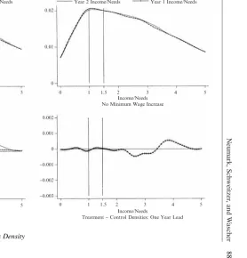
As a third check on our results, we looked for evidence of spurious “lead” effects of minimum-wage changes on the income-to-needs distribution. In particular, a poten-tial problem with any difference-in-difference estimator is that a different trend in the treatment group than in the control group can lead to a spurious inference about the treatment effect. In our case, if the difference-in-difference procedure generates results indicating that future minimum-wage increases lead to changes in the income-to-needs density, we might conclude that the estimates we reported in Figure 1 are confounding unspecified differential changes over time in the treatment and control groups with the true effects of minimum-wage increases. The results using one-year leads are displayed in Figure 3, and reveal no “effect” of future minimum-wage increases on the income-to-needs density.17
16. We do this analysis and the subsequent ones in this subsection for the baseline approach used in Figure 1, since the estimates with the fixed state and year effects were so similar.
Neumark, Schweitzer
, and W
ascher
887
Year 2 Income/Needs
Year 2 Income/Needs Year 1 Income/Needs Year 1 Income/Needs
0.02
0.002
0.001
0
−0.001
−0.002
−0.003
0.002
0.001
0
−0.001
−0.002
−0.003
0.01
0
0.02
0.01
0
1 1.5 2 3 4
0 5
1 1.5 2 3 4
0 5
1 1.5 2 3 4
0 5
Income/Needs
One Year Ahead of Minimum Wage Increase
Income/Needs Year 2 − Year 1 Densities
1 1.5 2 3 4
0 5
Income/Needs
Treatment − Control Densities: One Year Lead
Income/Needs No Minimum Wage Increase
Treatment Control
Figure 3
Finally, because our method is something of a “black box,” the credibility of our find-ing that minimum wages lead to increases in the proportion of poor or near-poor fami-lies would be strengthened by evidence indicating that low-wage workers suffer income declines when minimum wages increase. In this regard, evidence reported in Neumark, Schweitzer, and Wascher (2004b) shows that the adverse employment, hours, and income effects of minimum wages do indeed fall on workers earning near the minimum. In addition, Table 3 illustrates more clearly how families with incomes initially above the poverty or near-poverty line might be affected by an increase in the mini-mum wage. In particular, although minimini-mum-wage workers (those earning less than 110 percent of the minimum) account for a very small share of primary earners in fam-ilies above 1.5 times the poverty line (the second panel), it is not unusual for the low-est-paid worker in higher-income families to be paid at or below the minimum wage (the third panel). And as shown in the fourth panel, which presents the distribution of workers in each wage category across income-to-needs categories, there is nearly as large a proportion of minimum-wage workers (including those below the minimum) in families with incomes between 1.5 and 3 times the poverty line as between 0 and 1.5 times the poverty line, and actually a greater proportion of such workers in families with incomes-to-needs between 1.5 and 3 than below the poverty line.
Thus, the implication from Table 2 that minimum-wage increases cause some higher-income families to fall below the near-poverty line could easily reflect job losses among low-wage workers in these families,18 without implying any adverse impact on higher-wage workers. Moreover, the numbers of such secondary workers suggest that the magnitudes of the estimated effects reported in Table 2 are quite plau-sible. For example, about 22 percent of families with income-to-needs between 1.5 and 2 had at least two workers in our sample. In addition, as indicated in the third panel of Table 3, 51 percent of the secondary earners in this set of families earned less than 110 percent of the minimum. Thus, about 11 percent (22 percent ×.51) of fam-ilies in the 1.5–2 income-to-needs range had a worker who was paid close to the min-imum wage, and only a small share of these workers would have had to become disemployed to obtain the estimated 0.46 percentage point increase in the share of families with income-to-needs between 1 and 1.5 that is reported in Table 2.
Finally, to verify that the changes in the income-to-needs distribution are associated with relatively small declines in the incomes of families with low-wage workers, we also applied our difference-in-difference procedure for estimating the effects of min-imum wages to the distributions of changesin income-to-needs at different parts of the initial income-to-needs distribution. These estimates indicate that minimum-wage increases do not lead to a greater frequency of large declines in income-to-needs, but rather to a greater frequency of small declines in income-to-needs—specifically, declines of 0.5 or less.19 These results suggest that relatively few families with income-to-needs initially above 2 are falling into poverty. Instead, the observed changes in the income-to-needs distribution apparently come about because some families with income-to-needs of about 2 fall into the 1 to 1.5 interval, while others
18. In our data, we calculate that the incomes of nonprimary earners in these families are often quite low, with means of 5,700/7,500 (1982–84) dollars, and 25th centiles of 2,200 to 3,400 dollars.
with income-to-needs initially in the 1 to 1.5 range fall into poverty. That is, the esti-mated changes in the income-to-needs distribution shown in Figure 1 and Table 2 can be thought of as the cumulative effect of many families making small movements to the left in the distribution.
In our view, the variety of analyses in this subsection provide evidence that the results reported in Figure 1 and Table 2 represent the real effects of minimum wages, acting primarily through reduced employment opportunities or hours for low-wage workers.
V. Conclusions
In this paper, we attempt to address a central question regarding the wisdom of the minimum wage as social policy: Do minimum-wage increases raise the incomes of families at the lower end of the income distribution? Although modest dis-employment effects of minimum wages have often been interpreted as implying that minimum wages are likely to achieve this goal, there is little basis for this conclusion in the absence of direct evidence on the effects of the minimum wage on family incomes. The evidence we present comes from nonparametric difference-in-differ-ence estimates of the effects of minimum wages on the income-to-needs distribution and on the distribution of changes in income-to-needs.
Our results offer no empirical support for the hypothesis that minimum-wage increases reduce the proportions of poor and low-income families. The evidence on both family income distributions and changes in incomes experienced by families indicates that minimum wages raise the incomes of some poor families, but that the net effect of higher minimum wages is, if anything, to increase the proportions of families that are poor and near-poor. Thus, it would appear that reductionsin poverty or near-poverty should not be counted among the potential benefits of minimum wages. Returning to Gramlich’s question posed in the Introduction, our findings sug-gests that the efficiency and equity effects of minimum wages point in the same neg-ative direction.
Appendix 1
Contaminated Treatment and Control Groups
As noted in the text, we employ a procedure that uses all of the observations and dis-tributes the overall effects into “pure” contemporaneous and “pure” lagged effects correcting for the incidence of contaminated treatment and control groups. To explain the procedure, we first define the following terms:
C(I) = the estimated change in the density from Year 1 to Year 2 for observations with a contemporaneous increase in Year 2, versus the estimated change for observations with no contemporaneous increase,
L(I) = the similar estimate for lagged increases,
in(I) = the change in the density from Year 1 to Year 2 for observations with a contemporaneous increase in Year 2 and no lagged increase in Year 2,
ni(I) = the change in the density from Year 1 to Year 2 for observations with a lagged increase in Year 2 and no contemporaneous increase in Year 2,
ii(I) = the change in the density from Year 1 to Year 2 for observations with a contemporaneous increase in Year 2 and a lagged increase in Year 2,
nn(I) = the change in the density from Year 1 to Year 2 for observations with no contemporaneous increase in Year 2 and no lagged increase in Year 2,
Then C(I) is a weighted average of the estimated changes in densities over four groups:
(3) C(I) = α1{in(I) −nn(I)} + α2{in(I) −ni(I)} + α3{ii(I) −nn(I)}
+ α4{ii(I) −ni(I)},
where the first term corresponds to a change in densities estimated from uncontaminated treatment and control groups, the second term corresponds to an estimate with a con-taminated control group only, the third term corresponds to an estimate with a contam-inated treatment group only, and the fourth term corresponds to an estimate with a contaminated treatment and control group; the αk(which sum to 1) are the probabilities that the estimate comes from each of these groups.20Similarly, L(I) can be written as (4) L(I) = β1{ni(I) −nn(I)} + β2{ni(I) −in(I)} + β3{ii(I) −nn(I)}
+ β4{ii(I) −in(I)}.
Adding and subtracting nn(I) in the second and fourth terms in the equation for C(I), and assuming that
(5) {ii(I) −nn(I)} = {in(I) −nn(I)} +{ni(I) −nn(I)}, we can rewrite the expression for C(I) as
(6) C(I) = {in(I) −nn(I)} +(α3− α2) . {ni(I) −nn(I)}.
This expression makes intuitive sense. First, the final term in the equation for C(I) drops out because both the treatment and control group are contaminated, leaving the difference-in-difference estimate unaffected. Similarly, if α2= α3, so that there are equal likelihoods that the estimate comes from a contaminated treatment group (only) and a contaminated control group (only), the contamination again does not matter, and C(I) is the estimated change in the density for uncontaminated treatment and control groups. On the other hand, if α2< α3, so that there is a relatively higher probability of a contaminated treatment group, lagged effects {ni(I) −nn(I)} will be added to C(I), relative to the correct estimate of in(I) −nn(I). Conversely, if α2> α3, so that there is a relatively higher probability of a contaminated control group, lagged effects will be subtracted from C(I).
20. Define γas the probability that observations with a contemporaneous increase have a lagged increase as well (the probability that the treatment group is contaminated); this is estimated from the data. Similarly, define δas the probability that observations with no contemporaneous increase have a lagged increase (the probability that the control group is contaminated). Then assuming independence of the two types of con-tamination (because observations are either in the treatment or control group), α1= (1-γ)(1-δ), α2= (1-γ)δ,
In parallel fashion, L(I) can be rewritten as
(7) L(I) = {ni(I) −nn(I)} +(β3− β2) . {in(I) −nn(I)}.
We can solve the two equations C(I) and L(I) for the unknowns {in(I) −nn(I)} and {ni(I) −nn(I)}, which are the “pure” contemporaneous and lagged treatment effects, respectively, in which we are interested. Adding the “pure” lagged and contempora-neous effects together yields the combined “long-run” or “one-year-out” effect of minimum-wage increases on the income-to-needs density. In a regression framework with contemporaneous and lagged increases as independent variables, this would be equivalent to the sum of the contemporaneous and lagged effects.
The assumption embodied in Equation 5 merits some discussion. For the case in which all minimum-wage increases are of equal magnitude, this assumption means that the effect of two successive minimum-wage increases (relative to no increases for two years) is equal to the sum of a pure contemporaneous and a pure lagged increase. In a regression context, this is equivalent to the assumption that there is not an inter-action between contemporaneous and lagged effects.21
If, however, minimum-wage increases are of different sizes, as is actually the case, this assumption does not hold exactly. For example, many of the iiobservations—that is, those with a contemporaneous and lagged increase—are in 1991 and entail mini-mum-wage increases of $.45. In contrast, the $.90 increase in California contributes inand niobservations (in 1989 and 1990, respectively), but no iiobservations. On the other hand, there are also some smaller minimum-wage increases (for example, Oregon in 1994) that contribute inor niobservations. This problem reflects an inher-ent limitation of the nonparametric approach, which requires us to classify observa-tions as belonging to the treatment or control group, and does not permit us to exploit information on the size of the treatment.
Appendix 2
Bootstrapping Standard Errors and Confidence Intervals
The statistics of interest are all in the form of linear functions of density functions. The density estimates depend on both the households sampled within each state and the minimum-wage histories determined by the state of residence. Our bootstrapping procedure is designed to account for sampling variation in incomes and exposure to minimum-wage changes.
Neumark, Schweitzer, and Wascher 891
The statistics that we focus on are all extensions of difference-in-difference esti-mators like:
(8) S(I) = {f2,MW=1(I) −f1,MW=1(I)} −{f2,MW=0(I) −f1,MW=0(I)}.
All of the income-to-needs densities, f(I), are unknown and estimated using kernel density procedures on samples of households (j), with income-to-needs, sampling weights θj, and indicator variables for their state minimum-wage history and year in
the sampling frame Dj(that is, whether the observation is from a state-year observation
with a minimum-wage increase, and whether it is a Year 1 or a Year 2 observation). Thus, S(I) is estimated as:
(9) Se(I) = {fe(I⎪I
j, θj, Dj(year = 2,MW = 1)) −fe(I⎪Ij, θj, Dj
(year = 1, MW= 1))} −{fe(I⎪I
j, θj, Dj(year = 2, MW= 0)) −
fe(I⎪I
j, θj, Dj(year = 1, MW= 0))},
where, as in the text, the esuperscript denotes an estimate.
We are interested in using Se(I) to draw statistical inferences about the changes in
the density of income-to-needs induced by minimum-wage increases, whether at a particular value of I,or for a range of I(such as between 0 and 1). Although the his-tory of minimum-wage changes is known for all states, the composition of the sam-ple in each state is unknown, which is the source of randomness in the estimates. Each density function is estimated separately, but there are dependencies among the four densities in the expression for Se(I), making asymptotic standard errors based on the
individual densities unreliable. To address this we apply Efron’s bootstrapping proce-dure in the following way:
1. A random sample (b) is drawn from the data with replacement in order to replicate the realized overall sample sizes in every year, but allowing state-year sample sizes to vary.
2. Sets of estimates of all densities are calculated for each bootstrap sample. The statistics of interest are calculated based on each of these densities.
3. This process is repeated Btimes.
If Se(I) is the estimate corrected for contaminated contemporaneous and lagged
effects, as discussed in the text, then the test of the hypothesis that the effect of a min-imum-wage change on frequencies of income/needs over an interval (α, β] is greater than or equal to zero is whether
(10) Pe(S(I) ≥0 ⎪ α< I≤ β) = #(Σ
Iε(α,β]S(I) ≥0)/B
is statistically significantly greater than zero, where # represents a count of cases sat-isfying the inequality. If Se(I) tended to cross the zero axis in the tested range, the null
hypothesis would be less likely to be rejected.
Alternatively, focusing on the point estimates of effects at a particular income-to-needs level Iincreases the uncertainty of the estimates, because less effective data (judged by the sum of kernel weights at the point) are entered into the calculation. The
γpercent confidence interval for the estimated S(I) is simply the range of central γ per-cent of Se(I)
not be symmetric. Accurate confidence intervals of this type require a large number of bootstrap repetitions (at least 500).
The reliability of bootstrap standard errors for kernel density estimates has been criticized by Hall (1992) because kernel density estimates are inherently biased. The bias for the Gaussian kernel used in our results is
(11) Bias fe(I) = 1/2h2f ′′(I),
where h is the bandwidth. The effect of this bias is to understate a rapid change in the frequency of observations. The bootstrap applied directly to the estimator does not account for this bias, so it may estimate confidence intervals with incom-plete coverage. The bias problem of kernel density estimates, and the related under-coverage of bootstrap standard errors, diminishes as the sample size rises (and the optimal bandwidth declines) or when the underlying data is smooth. Alternative approaches for generating bootstrap confidence intervals have been suggested by Hall (1992) and Chen (1996). However, practical guidance on using these techniques based on Monte Carlo simulations recommends that more sophisticated methods to correct for the bias be used only when the sample sizes are smaller than 100 in any of the samples being compared (Handcock and Morris 1998). In our case, the samples for each of the comparison groups always number in the tens of thousands.
There are additional reasons to think that the bias would be small in our particular application. For example, our statistics involve paired differences where the underly-ing distributions of family incomes are similarly smooth and have similar shapes, so that any kernel density estimation biases are likely to partially cancel out. In addition, we apply adaptive smoothing techniques–reducing the bandwidth where the sample sizes are relatively large–to further reduce the bias in the area of interest (near the poverty level).
References
Addison, John T., and McKinley L. Blackburn. 1999. “Minimum Wages and Poverty.”
Industrial and Labor Relations Review52(3):393–409.
Baker, Michael, Dwayne Benjamin, and Shuchita Stanger. 1999. “The Highs and Lows of the Minimum Wage Effect: A Time-Series Cross-Section Study of the Canadian Law.” Journal of Labor Economics17(2):318–50.
Brown, Charles, Curtis Gilroy, and Andrew Kohen. 1982. “The Effect of the Minimum Wage on Employment and Unemployment.” Journal of Economic Literature20(2):487–528. Burkhauser, Richard V., Kenneth A. Couch, and David C. Wittenburg. 1996. “ ‘Who Gets
What’ from Minimum Wage Hikes: A Re-Estimation of Card and Krueger’s Distributional Analysis in Myth and Measurement: The New Economics of the Minimum Wage.” Industrial and Labor Relations Review49(3):547–52.
Burkhauser, Richard V., and T. Aldrich Finegan. 1989. “The Minimum Wage and the Poor: The End of a Relationship.” Journal of Policy Analysis and Management8(1):53–71. Card, David. 1992. “Using Regional Variation in Wages to Measure the Effects of the Federal
Minimum Wage.” Industrial and Labor Relations Review46(1):22–37.
Card, David, and Alan B. Krueger. 1995. Myth and Measurement: The New Economics of the Minimum Wage. Princeton, N. J.: Princeton University Press.
Chen, Song Xi. 1996. “Empirical Likelihood Confidence Intervals for Nonparametric Density Estimation.” Biometrika83(2):329–41.
Connolly, Laura S., and Lewis M. Segal. 1997. “Minimum Wage Legislation and the Working Poor.” Chicago: Federal Reserve Bank of Chicago. Unpublished.
Cushing, Brian. 2003. “State Minimum Wage Laws and the Migration of the Poor.” Research Paper 2003-3, Department of Economics. Morgantown: West Virginia University.
DiNardo, John, Nicole M. Fortin, and Thomas Lemieux. 1996. “Labor Market Institutions and the Distribution of Wages, 1973–1992: A Semiparametric Approach.” Econometrica
64(5):1001–44.
Freeman, Richard B. 1996. “The Minimum Wage as a Redistributive Tool.” Economic Journal
106(436):639–49.
Gelbach, Jonah B. 2004. “Migration, the Life Cycle, and State Benefits: How Low is the Bottom?” Journal of Political Economy112(5):1091–130.
Gramlich, Edward M. 1976. “Impact of Minimum Wages on Other Wages, Employment, and Family Incomes.” Brookings Paper on Economic Activity1:409–51.
Hall, Peter. 1992. The Bootstrap and the Edgeworth Expansion. New York: Springer-Verlag. Handcock, Mark S., and Martina Morris. 1998. “Relative Distribution Methods.” Sociological
Methods28:53–97.
Hamermesh, Daniel S. 1993. Labor Demand. Princeton, N.J.: Princeton University Press. Härdle, Wolfgang. 1991. Smoothing Techniques: With Implementation in S. New York:
Springer-Verlag.
Horrigan, Michael W., and Ronald B. Mincy. 1993. “The Minimum Wage and Earnings and Income Inequality.” In Uneven Tides: Rising Inequality in America, ed. Sheldon Danziger and Peter Gottschalk, 251–75. New York: Russell Sage Foundation.
Hungerford, Thomas L. 1996. “Does Increasing the Minimum Wage Increase the Proportion of Involuntary Part-Time Workers?” Washington, D.C.: U.S. General Accounting Office. Unpublished.
Johnson, William R., and Edgar K. Browning. 1983. “The Distributional and Efficiency Effects of Increasing the Minimum Wage: A Simulation.” American Economic Review
73(1):204–11.
Marron, J. S. and H. P. Schmitz. 1992. “Simultaneous Density Estimation of Several Income Distributions.” Econometric Theory8(4):476–88.
Neumark, David, Mark Schweitzer, and William Wascher. 2004a. “The Effects of Minimum Wages on the Distribution of Family Incomes: A Non-Parametric Analysis.” Federal Reserve Bank of Cleveland Working Paper No. 04-12. Cleveland: Federal Reserve Bank of Cleveland.
Neumark, David, Mark Schweitzer, and William Wascher. 2004b. “Minimum Wage Effects Throughout the Wage Distribution.” Journal of Human Resources39(2):425–50. Neumark, David, and William Wascher. 2002. “Do Minimum Wages Fight Poverty?”
Economic Inquiry40(3):315–33.
. 1992. “Employment Effects of Minimum and Subminimum Wages: Panel Data on State Minimum Wage Laws.” Industrial and Labor Relations Review46(1):55–81. Silverman, B. W. 1986. Density Estimation for Statistics and Data Analysis. London:
Chapman and Hall.