Manajemen | Fakultas Ekonomi Universitas Maritim Raja Ali Haji 373.full

Guido W. Imbens is a professor of economics at the Stanford Graduate School of Business. Some data used in this article are available from the author beginning November 2015 through October 2018.

[Submitted March 2013; accepted March 2014]

ISSN 0022- 166X E- ISSN 1548- 8004 © 2015 by the Board of Regents of the University of Wisconsin System

T H E J O U R N A L O F H U M A N R E S O U R C E S • 50 • 2

Three Examples

Guido W. Imbens

Imbens

abstract

There is a large theoretical literature on methods for estimating causal effects under unconfoundedness, exogeneity, or selection- on- observables type assumptions using matching or propensity score methods. Much of this literature is highly technical and has not made inroads into empirical practice where many researchers continue to use simple methods such as ordinary least squares regression even in settings where those methods do not have attractive properties. In this paper, I discuss some of the lessons for practice from the theoretical literature and provide detailed recommendations on what to do. I illustrate the recommendations with three detailed applications.

I. Introduction

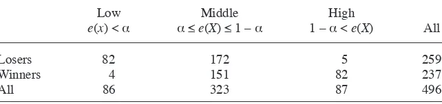
In this paper, I provide some advice for researchers estimating average treatment ef-fects in practice, based on my personal view of this literature. The issues raised in this paper draw from my earlier reviews (Imbens 2004; Imbens and Wooldridge 2009) and in particular my forthcoming book with Imbens and Rubin (2015) and research papers (in particular, Abadie and Imbens 2006, 2008; Hirano, Imbens, and Ridder 2003). I focus on four speci_fi c issues. First, I discuss when and why the simple ordinary least squares estimator, which ultimately relies on the same fundamental unconfoundedness assump-tion as matching and propensity score estimators, but which combines that assumpassump-tion with strong functional form restrictions, is likely to be inadequate for estimating average treatment effects. Second, I discuss in detail two speci_fi c, fully speci_fi ed, estimators that in my view are attractive alternatives to least squares estimators because of their robustness properties with respect to a variety of data con_fi gurations. Although I focus on these two methods, one based on matching and one based on subclassi_fi cation on the propensity score, in some detail, the message emphatically is not that these are the only two estimators that are reasonable. Rather, the point is that the results should not be sensitive to the choice of reasonable estimators, and that unless a particular estimator is robust to modest changes in the implementation, any results should be viewed with suspicion. Third, I discuss trim-ming and other preprocessing methods for creating more balanced samples as an important fi rst step in the analysis to ensure that the _fi nal results are more robust with any estimators, including least squares, weighting, or matching. Fourth, I discuss some supplementary analyses for assessing the plausibility of the unconfoundedness assumption. Although unconfoundedness is not testable, one should assess, whenever possible, whether uncon-foundedness is plausible in speci_fi c applications, and in many cases one can in fact do so. I illustrate the methods discussed in this paper using three different data sets. The _fi rst of these is a subset of the lottery data collected by Imbens, Rubin, and Sacerdote (2001). The second data set is the experimental part of the Dehejia and Wahba (1999) version of the Lalonde (1986) data set containing information on participants in the Nation-ally Supported Work (NSW) program and members of the randomized control group. The third data set contains information on participants in the NSW program and one of Lalonde’s nonexperimental comparison groups, again using the Dehejia- Wahba version of the data. Both subsets of the Dehejia- Wahba version of the Lalonde data are available on Dehejia’s website, http://users.nber.org/rdehejia/. Software for implementing these methods will be available on my website.

II. Setup and Notation

The setup used in the current paper is by now the standard one in this literature, using the potential outcome framework for causal inference that builds on Fisher (1925) and Neyman (1923) and was extended to observational studies by Rubin (1974). See Imbens and Wooldridge (2009) for a recent survey and historical context, and Imbens and Rubin (2014) for the speci_fi c notation used here. Following Holland (1986), I will refer to this setup as the Rubin Causal Model, RCM for short.1

The analysis is based on a sample of N units, indexed by i = 1, . . . , N, viewed as a random sample from an in_fi nitely large population.2 _{For unit i, there are two potential} outcomes, denoted by Y_i(0) and Y_i(1), the potential outcomes without and given the treatment respectively. Each unit in the sample is observed to receive or not receive a binary treatment, with the treatment indicator denoted by W_i. If unit i receives the treatment, then W_i = 1, otherwise W_i = 0. There are N_{c =} ⌺i=1

N

(1−Wi) control units and

N_{t =} ⌺i=1 N

(1−Wi) treated units, so that N = N_c + N_t is the total number of units. The realized (and observed) outcome for unit i is

Y_iobs

=Y_i(W_i)=

Y_{i(0) if}W_i=0

Y_{i(1) if}W_{i =1} ⎧

⎨ ⎪

⎩⎪ .

I use the superscript “obs” here to distinguish between the potential outcomes that are not always observed and the observed outcome. In addition, there is for each unit i a

K- component covariate X_i, with X_i∈_⺨ ⊂_⺢K_{. The key characteristic of these} covari-ates is that they are known not to be affected by the treatment. Observe that, for all units in the sample, the triple (Y_iobs

,W_i,Xi). We use Y, W, and X to denote the vectors with tyical elements Yobsi and W_i, and the matrix with i- th row equal to Xi′.

De_fi ne the population average treatment effect conditional on the covariates,

␶(x_)=⺕[Y_i(1)−Y_i(0)|X_i= x],

and the average effect in the population, and in the subpopulation of treated units,

(1) ␶ _=⺕[Y_i(1)−Y_{i(0)], and} ␶_{treat =⺕}[Y_i(1)−Y_i(0)|W_i=1]

There is a somewhat subtle issue that can also be focused on the sample average treat-ment effects, conditional on the covariates in the sample,

(2) ␶sample = 1

N _i ␶(Xi)

=1 N

∑

, and ␶treat,sample =

1

N_t ␶(Xi)

i:Wi=1

∑

.

This matters for inference, although not for estimation. The asymptotic variances for the same estimators, viewed as estimators of ␶_sample and ␶_treat,sample, are generally smaller than when we view _␶ and ␶_treat as the target, unless there is no variation in ␶(x) over the population distribution of X_i. See Imbens and Wooldridge (2009) for more details on this distinction.

The _fi rst key assumption made is unconfoundedness (Rubin 1990), (3) W_i⊥ ₍Y_i(0),Y_i(1))|X_i,

where, using the Dawid (1979) conditional independence notation, A⊥ B_|C denotes that A and B are independent conditional on C. The second key assumption is overlap, (4) 0<e₍x_)<1,

for all x in the support of the covariates, where (5) e₍x_)=⺕[W_i|X_i= x_{]= Pr(}W_i=1|X_{i =} x),

is the propensity score (Rosenbaum and Rubin 1983). The combination of these two assumptions is referred to as strong ignorability by Rosenbaum and Rubin (1983). The combination implies that the average effects can be estimated by adjusting for differ-ence in covariates between treated and control units. For example, given unconfound-edness, the population average treatment effect _␶ can be expressed in terms of the joint distribution of (Y_iobs

,W_i,X_i) as

(6) ␶ _=⺕[⺕[Yobsi_|W

i =1,Xi]−⺕[Yobsi|Wi =0,Xi]].

To see that Equation 6 holds, note that by de_fi nition,

⺕[⺕[Y_iobs

|W_i=1,X_i]−_⺕[Y_iobs

|W_{i =0,}X_i]]=⺕[⺕[Y_i(1)|W_i=1,X_i]−_⺕[Y_i(0)|W_{i =0,}X_i]]. By unconfoundedness, the conditioning on W_i in these two terms can be dropped, and

⺕[⺕[Y_i(1)|W_i=1,X_i]−_⺕[Y_i(0)|W_{i =0,}X_i]]=⺕[⺕[Y_i(1)|X_i]−_⺕[Y_i(0)|X_i]] =⺕[⺕[Y_i(1)−Y_i(0)|X_i]]=␶, thus proving Equation 6.

To implement estimators based on this equality, it is also required that the condi-tional expectations _⺕[Y_i(0)|X_{i =} x_], _⺕[Y_i(1)|X_i= x] and e(x) are suf_fi ciently smooth— that is, suf_fi ciently many times differentiable. See the technical papers in this litera-ture, referenced in Imbens and Wooldridge (2009), for details on the smoothness requirements.

The statistical challenge is now how to estimate objects such as

(7) _⺕[⺕[Y_iobs

|W_i=1,X_i]−_⺕[Y_iobs

|W_{i =0,}X_i]].

One would like to estimate Equation 7 without relying on strong functional form as-sumptions on the conditional distributions or conditional expectations. One would also like the estimators to be robust to minor changes in the implementation of the estimator. Whether these two assumptions are reasonable is often controversial. Violations of the overlap assumptions are often easily detected. They motivate some of the design issues and often imply that the researcher should change the estimand from the overall average treatment effect to an average for some subpopulation. See Section VF for more discussion. Potential violations of the unconfoundedness assumption are more dif_fi cult to address. First, there are some methods for assessing the plausibility of the assumption, see the discussion in Section VG. To make the assumption plausible, it is important to have detailed information about the units on characteristics that are associated both with the potential outcomes and the treatment indicator. It is often particularly helpful to have lagged measures of the outcome, for example, detailed labor market histories in evaluations of labor market programs. At the same time, hav-ing detailed information on the background of the units makes the statistical challenge of adjusting for all these differences more challenging.

Fraser (2010); and Murnane and Willett (2010). Much of the econometrics literature is technical in nature and has primarily focused on establishing _fi rst- order large- sample properties of point and interval estimators using matching (Abadie and Imbens 2006), nonparametric regression methods (Frolich 2000; Chen, Hong, and Tarozzi 2008; Hahn 1998; Hahn and Ridder 2013), or weighting (Hirano, Imbens, and Ridder 2003; Frölich 2002). These _fi rst- order asymptotic properties are identical for a number of proposed methods, limiting the usefulness of these results for choosing between these methods. In addition, comparisons between the various methods based on Monte Carlo evidence (for example, Frölich 2004; Busso, DiNardo, and McCrary 2008; Lechner 2012) are ham-pered by the dependence of many of the proposed methods on tuning parameters (for example, the bandwidth choices in kernel regression, or on the number of terms or basis functions in sieve or series methods) for which rarely speci_fi c, data- dependent values are recommended, as well as by the lack of agreement on realistic designs in simulation studies.

In this paper, I will discuss my recommendations for empirical practice based on my reading of this literature. These recommendations are somewhat personal. In places they are also somewhat vague. I will emphatically not argue that one particular estima-tor should always be used. Part of the message is that there are no, and will not be, general results implying that in general some estimators are superior to all others. The recommendations are more speci_fi c in other places—for example suggesting supple-mentary analyses that indicate for some data sets that particular estimators will be sen-sitive to minor changes in implementation—thus making them unattractive in those settings. The hope is that these comments will be useful for empirical researchers. The recommendations will consist of a combination of particular estimators, supplemen-tary analyses, and, perhaps most controversially, changes in estimands when Equation 7 is particularly dif_fi cult to estimate.

III. Least Squares Estimation: When and Why Does It

Not Work?

The most widely used method for estimating causal effects remains ordinary least squares (OLS) estimation. Ordinary least squares estimation relies on unconfoundedness in combination with functional form assumptions. Typically, re-searchers make these functional form assumptions for convenience, viewing them at best as approximations to the underlying functions. In this section, I discuss merits and concerns with this method for estimating causal effects as opposed to using it for prediction. The main point is that the least squares functional form assumptions matter, and sometimes matter substantially. Moreover, one can assess from the data whether this will be the case.

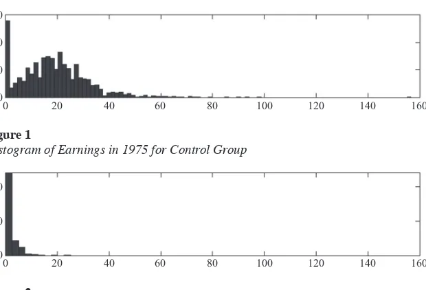
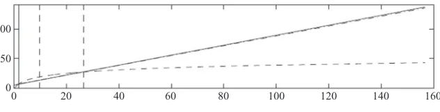
covariate, earn’75. There are N_t = 185 men in the treatment group and N_c = 2,490 men in the control group. From the experimental data, it can be inferred that the average causal effect is approximately $2,000. Figures 1 and 2 present histograms of earn’75 in the control and treatment group respectively. The average values of this variable in the two groups are 19.1 and 1.5, with standard deviations 13.6 and 3.2 respectively. Clearly, the two distributions of earn’75 in the trainee and comparison groups are far apart.

A. Ordinary Least Squares Estimation

Initially, I focus on the average effect for the treated, ␶_treat, de_fi ned in Equation 1, al-though the same issues arise for the average effect _␶. Focusing on ␶_treat simpli_fi es some of the analytic calculations. Under unconfoundedness, ␶_treat can be written as a func-tional of the joint distribution of (Y_iobs

,W_i,X_i)—that is,

(8) ␶_treat =⺕[Y_iobs

|W_{i =1]}−_⺕[⺕[Y_iobs

|W_{i =0,}X_i]|W_i=1].

De_fi ne

Y_cobs

= 1

N_c

Y_iobs i:Wi

∑

=0

, Y_tobs

= 1

N_t =

Y_iobs i:Wi

∑

=1

X_{c =} 1

N_c Xi

i:Wi

∑

=0

, and X_t= 1

N_t Xi

i:Wi

∑

=1 .

The _fi rst term in Equation 8, _⺕[Y_iobs

|W_{i =1]}, is directly estimable from the data as Y_t. It is the second term, ⺕[⺕[Y_iobs

|W_i=0,X_i]|W_{i =1]}, that is more dif_fi cult to estimate. Suppose we specify a linear model for Y_i(0) given X_i:

300

200

100

0

0 20 40 60 80 100 120 140 160

100

50

0

0 20 40 60 80 100 120 140 160

Figure 1

Histogram of Earnings in 1975 for Control Group

Figure 2

⺕[Y_i(0)|X_i= x_]= ␣c+␤c⋅x.

The OLS estimator for ␤c is equal to

ˆ

␤c =

⌺i:Wi=0(Xi− Xc)⋅(Yi

obs−_Y

c obs

)

⌺i:Wi=0(Xi− Xc)2

, and ˆ␣c =Yc obs−_␤ˆ

c⋅Xc.

For the Lalonde nonexperimental data, where the outcome is earnings in thousands of dollars, and the scalar covariate here lagged earnings, we have

ˆ

␤c =0.84 (s.e. 0.03), ˆ␣c =5.60 (s.e. 0.51).

Then, we can write the OLS estimator of the average of the potential control outcomes for the treated, ⺕[Y_i(0)|W_i=1], as

(9) ⺕[Y_i(0)|pW_i=1]=Y_c+␤ˆc⋅(Xt− Xc),

which for the Lalonde data leads to

⺕[Y_i(0)|pW_{i =1]=6.88 (s.e. 0.48)}.

The question is how credible this is as an estimate of ⺕[Y_i(0)|W_i=1]. I focus on two as-pects of this credibility.

B. Extrapolation and Misspecifi cation

First, some additional notation is needed. Denote the true conditional expectation and variance of Y_i(w) given X_i = x by

␮w(x_)=⺕[Y_i(w_)|X_i= x_{], and} ␴w2(x)=⺦(Yi(w)|Xi= x).

Given the true conditional expectation, the pseudotrue values for ␤c, the probability

limit of the OLS estimator, is

␤c*= plim( ˆ␤c)= ⺕

[␮c(X_i)⋅₍X_i−_⺕[X_i])|W_i=0]

⺕[(X_i−_⺕[X_i])2_|W

i= 0]

,

and the estimator for the predicted value for ⺕[Y_i(0)|W_i=1] will converge to

plim(⺕[Y_i(0)|pW_{i =1])=⺕[}Y_i(0)|W_{i =0]+}␤c

*⋅_(⺕[Xi|W

i =1]−⺕[Xi|Wi= 0]). =⺕[Y_i(0)|W_i=1]−_(⺕[␮t(X_i)|W_i=1]−_⺕[␮t(X_i)|W_{i= 0])}

+␤c

*_⋅(

⺕[X_i|W_i=1]−_⺕[X_i|W_{i =0]).}

The difference between the plim(⺕[Y_i(0)|pW_i=1]) and the true average _⺕[Y_i(0)|W_{i =1]} depends on the difference between the average value of the regression function for the treated and the controls and the approximation of this difference of the average condi-tional expectations by the difference in the average values of the best linear predictors,

plim(⺕[Y_i(0)|pW_i=1])−_⺕[Y_i(0)|W_i=1]

=␤c

*⋅₍

fx(x|Wi= 0)= fx(x|Wi =1) for all x, the difference is zero. However, if both the con-ditional expectations are nonlinear and the covariate distributions differ, there will in general be a bias. Establishing whether the conditional expectations are nonlinear can be dif_fi cult to do. However, it is straightforward to assess whether the second neces-sary condition for bias is satis_fi ed, namely whether the distributions of the covariates in the two treatment arms are similar or not.

Now look at the sensitivity to different speci_fi cations. I consider two speci_fi cations for the regression function. First, a simple linear regression:

earn′78= ␣_c+␤_c⋅earn′75+␧_i (linear).

Second, a linear regression after transforming the regressor by adding one unit ($1,000) followed by taking logarithms:

earn′78=␣_c+␤_c⋅ln(1+earn′75)+␧_i (log linear).

The predictions for ⺕[Yi(0)|Wi=1] based on the two models are quite different, given that the average causal effect is on the order of $2,000:

⺕[Yi(0)|pWi=1]linear =6.88 (s.e. 0.48) ⺕[Yi(0)|pWi=1]loglinear = 2.81 (s.e. 0.66).

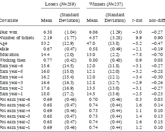
The reason for the big difference (4.07) between the two predicted values can be seen in Figure 3 where I plot the two estimated regression functions. The dashed vertical lines present the 0.25 and 0.75 quartile of the distribution of earn’75 for the PSID sample (9.84 and 24.50 respectively). This indicates the range of values where the regression function is most likely to approximate the conditional expectation accurately. The solid vertical lines present the 0.25 and 0.75 quantiles for the distribution of earn’75 for the trainees (0 and 1.82 respectively). One can see in this fi gure that for the range where the trainees are and where we therefore need to predict Y_i(0), with earn’75 between 0 and 1.82, the predictions of the linear and the log- linear model are quite different.

The estimates here were based on regression outcomes on earnings in 1975 for the control units only. In practice, an even more common approach is to simply estimate the regression

earn′78= ␣+␶⋅Wi+␤⋅earn′75+␧i (linear), or

earn′78 =␣+␶⋅Wi+␤c⋅ln(1+earn′75)+␧i (log linear), Figure 3

Linear and Log Linear Regression Functions, and Quartiles of Earnings Distributions

100

50

0

on the full sample, including both treated and control units. The reason for focus-ing on the regression in the control sample here is mainly expositional: It simpli_fi es the expressions for the estimated average of the potential outcomes. In practice, it makes relatively little difference if we do the regressions with both treated and control units included. For these data, with many more control units (2,490) than treated units (1,985), the estimates for the average of the potential outcome Y_i(0) for the treated are, under the linear and log linear model, largely driving by the values for the control units. Estimating the regression function as a single regression on all units leads to:

⺕[Y_i(0)|pW_i=1]

linear,full sample =6.93 (s.e. 0.47)

⺕[Y_i(0)|pW_{i =1]}

log linear,full sample =3.47 (s.e. 0.38),

with the difference in the average predicted value for Y_i(0) for the treated units be-tween the linear and the log linear specifi cation much bigger than between the regres-sion on the control sample versus the regresregres-sion on the full sample.

C. Weights

Here, I present a different way of looking at the sensitivity of the least squares estima-tor in settings with substantial differences in the covariates distributions. One can write the OLS estimator of _⺕[Y_i(0)|W_i=1] in a different way, as

(10) ⺕[Y_i(0)|pW_i=1]= 1 N_ci ␻i

:Wi

∑

=0

⋅Y_iobs_,

where, for control unit i the weight ␻i is

(11) ␻i =1−(Xi− Xc)⋅

X_c− X_t

X2−_X ⋅ _X.

It is interesting to explore the properties of these weights ␻i. First, the weights average to

one over the control sample, irrespective of the data. Thus, ⺕[Y_i(0)|pW_{i =}1] is a weighted average of the outcomes for the control units, with the weights adding up to 1. Second, the normalized weights ␻i are all equal to one in the special case where the average of the

covariates in the two groups are indentical. In that case, _⺕[Y_i(0)|pW_{i =1]=}Y_cobs_{. In a}

ran-domized experiment, X_c is equal to X_t in expectation, so the weights should be close to one in that case. The variation in the weights, and the possibility of relatively extreme weights, increases with the difference between X_c and X_t. Finally, note that given a par-ticular data set, one can inspect these weights directly and assess if some units have exces-sively large weights.

Let us _fi rst look at the normalized weights ␻i for the Lalonde data. For these data,

the weights take the form

␻i= 2.8091−0.0949⋅Xi.

The average of the weights is, by construction, equal to 1. The standard deviation of the weights is 1.29. The largest positive weight is 2.08, for control units with earn’75

earn’75 equal to 156.7, with a weight of –12.05. This is where the problem with ordi-nary least squares regression shows itself most clearly. The range of values of earn’75

for trainees is [0,25.14]. I would argue that whether an individual with earn’75 equal to $156,700 makes $100,000 or $300,000 in 1978 should make no difference for a predic-tion for the average value of Y_i(0) for the trainees in the program, _⺕[Y

i(0)|Wi =1], given

that the maximum value for earn’75 for trainees is $25,140. Conditional on the speci-fi cation of the linear model, however, that difference between $100,000 and $300,000 is very important for the prediction of earnings in 1978 for trainees. Given the weight of –12.05 for the control individual with earn’75 equal to 156.7, the prediction for

⺕[Y

i(0)|Wi=1] would be 6.829 if earn’78 = 100 for this individual, and 5.861 if earn’78

= 300 for this individual, with the difference equal to $968, a substantial amount. The problem is that the least squares estimates take the linearity in the linear regression model very seriously, and, given linearity, observations on units with extreme values for

earn’75 are in fact very informative. Note that one can carry out these calculations without even using the outcome data. Because the weights are so large, the value of

earn’78 for such individuals matters substantially for our prediction for ⺕[Y

i(0)|Wi=1],

where arguably the earnings for such individuals should have close to 0 weight.

D. How to Think About Regression Adjustment

Of course, the example in the previous subsection is fairly extreme. The two distribu-tions are very different with, for example, the fraction of the PSID control sample with

earn’75 exceeding the maximum value found in the trainee sample (which is 25.14) equal to 0.27. It would appear obvious that units with earn’75 as large as 156.7 should be given little or no weight in the analyses. An obvious remedy would be to discard all PSID units with earn’75 exceeding 25.14, and this would go a considerable way to-ward making the estimators more robust. However, it is partly because there is only a single covariate in this overly simplistic example that there are such simple remedies.3 With multiple covariates, it is dif_fi cult to see what trimming would need to be done. Moreover, a simple trimming rule such as the one described above is very sensitive to outliers. If there were a single trainee with earn’75 equal to 150, that would change the estimates substantially. The issue is that regression methods are fundamentally not robust to the substantial differences between treatment and control groups. I will be discussing alternatives to the simple regression methods used here that do systemati-cally, and automatisystemati-cally, down weight the in_fl uence of such outliers, both in the case with scalar covariates and in the case with multivariate covariates. If, for example, instead of using regression methods, one matched all the treated units, the control units with earn’75 exceeding 25.07 would receive 0 weight in the estimation, and in fact few control units with earn’75 between 18 and 25 would receive positive weights. Matching is therefore by design robust to the presence of such units.

In practice, it may be useful to compare the least squares estimates to estimates based on more sophisticated methods, both as a check that calculations were car-ried out correctly and to ensure that one understands what is driving any difference between the estimates.

IV. The Strategy

In this section, I lay out the overall strategy for _fl exibly and robustly estimating the average effect of the treatment. The strategy will consist of two and sometimes three distinct stages, as outlined in Imbens and Rubin (2015). In the _fi rst stage, which, following Rubin (2005), I will refer to as the design stage, the full sample will be trimmed by discarding some units to improve overlap in covariate distributions. In the second stage, the supplementary analysis stage, the unconfound-edness assumption is assessed. In the third stage, the analysis stage, the estimator for the average effect will be applied to the trimmed data set. Let me brie_fl y discuss the three stages in more detail.

A. Stage I: Design

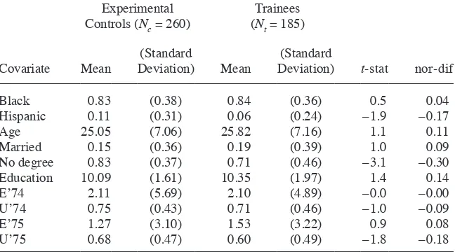
In this stage, we do not use the outcome data and focus solely on the treatment indica-tors and covariates, (X,W). The _fi rst step is to assess overlap in covariate distributions. If this is found to be lacking, a subsample is created with more overlap by discarding some units from the original sample. The assessment of the degree of overlap is based on an inspection of some summary statistics, what I refer to as normalized differences in covariates, denoted by ⌬X. These are differences in average covariate values by treatment status, scaled by a measure of the standard deviation of the covariates. These normalized differences contrast with t- statistics for testing the null of no differences in means between treated and controls. The normalized differences provide a scale and sample size free way of assessing overlap.

If the covariates are far apart in terms of this normalized difference metric, one may wish to change the target. Instead of focusing on the overall average treatment effect, one may wish to drop units with values of the covariates such that they have no counterparts in the other treatment group. The reason is that, in general, no estimation procedure will be given robust estimates of the average treatment effect in that case. To be speci_fi c, following Crump, Hotz, Imbens, and Mitnik (2008a, CHIM from hereon), I propose a rule for drop-ping units with extreme (that is, close to 0 or 1) values for the estimated propensity score. This step will require estimating the propensity score eˆ₍x_:W_,X_{). One can capture the}

result of this _fi rst stage in terms of a function I = I(W, X) that determines which units are dropped as a function of the vector of treatment indicators W and the matrix of pretreat-ment variables X. Here, I denotes an N vector of binary indicators, with i- th element I_i

equal to one if unit i is included in the analysis, and I_i equal to zero if unit i is dropped. Dropping the units with I_i = 0 leads to a trimmed sample (YT_,WT_{, X}T_{) with} N

s= ⌺i₌1 N _{Ii units.}

B. Stage II: Supplementary Analysis: Assessing Unconfoundedness

will involve _fi rst trimming this pseudosample using the same procedures to construct a trimmed sample (X

p T_,WT_,X

rT) and then estimating a “pseudo” average treatment

effect on the pseudo- outcome for this trimmed sample. Speci_fi cally, I calculate

ˆ ␶_{X =}␶(X

p T_,WT_,X

rT)

for speci_fi c estimators ␶(⋅) described below, where the adjustment is only for the subset of covariates included in X_rT_{. This estimates the “pseudo” causal effect, the causal}

ef-fect of the treatment on the pretreatment variable X

p

T_{, which is a priori known to be}

zero. If we _fi nd the estimate ␶ˆ_X is substantially and statistically close to zero after ad-justing for X_rT_{, this will be interpreted as evidence supportive of the assumption of}

unconfoundedness. If the estimate ␶ˆ_X differs from zero, either substantially or statisti-cally, this will be viewed as casting doubt on the (ultimately untestable) unconfound-edness assumption, with the degree of evidence dependent on the magnitude of the deviations. The result of this stage will therefore be an assessment of the credibility of any estimates of the average effect of the treatment on the outcome of interest, without using the actual outcome data.

C. Stage III: Analysis

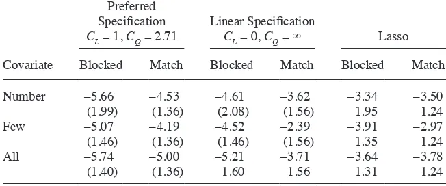
In the third stage, the outcome data Y are used and estimates of the average treatment effect of interest are calculated. Using one of the recommended estimators, block-ing (subclassi_fi cation) or matching, applied to the trimmed sample, we obtain a point estimate:

ˆ

␶ ₌␶(YT_,WT_,XT_).

This step is more delicate, with concerns about pretesting bias, and I therefore propose no speci_fi cation searches at this stage. The _fi rst estimator I discuss in detail is based on blocking or subclassi_fi cation on the estimated propensity score in combination with regression adjustments within the blocks. The second estimator is based on direct one- to- one (or one- to- k) covariate matching with replacement in combination with regres-sion adjustments within the matched pairs. Both are, in my view, attractive estimators because of their robustness.

V. Tools

In this section, I will describe the calculation of the normalized differ-ences ⌬_X,k and the four functions—the propensity score, e(x;W, X), the trimming func-tion, I(W, X), the blocking estimator, ␶_block(Y_,W_,X_{), and the matching estimator,} ␶_match(Y_,W_,X_{)—and the choices that go into these functions.}

such as age should enter linearly or quadratically in the propensity score in the context of the evaluation of a labor market program. The methods described here are intended to assist the researcher in such decisions by providing a benchmark estimator for the average effect of interest.

A. Assessing Overlap: Normalized Differences in Average Covariates

For element X_i,k of the covariate vector X_i, the normalized difference is de_fi ned as

(12) ⌬_X,k = Xt,k −Xc,k (S

X,t,k 2

+S

X,t,k 2 _{) / 2}

where

X

c,k =

1 N_c

X

i,k,Xt,k i:Wi=

∑

0

= 1 N_t

X

i,k i:Wi=

∑

1

,

S_X,c,k2

= 1

N_c−1 (Xi,k −Xc,k)

2

i:Wi=0

∑

, and S_X,t,k2

= 1

N_t−1 (Xi,k −Xt,k)

2

i:Wi=1

∑

.

A key point is that the normalized difference is more useful for assessing the magni-tude of the statistical challenge in adjusting for covariate differences between treated and control units than the t- statistic for testing the null hypothesis that the two differ-ences are zero, or

(13) t

X,k =

X

t,k− Xc,k

S

X,t,k

2 _{/ N}

t+SX,c,k

2 _/N

c

.

The t- statistic t_X,k may be large in absolute value simply because the sample is large and, as a result, small differences between the two sample means are statistically signif-icant even if they are substantively small. Large values for the normalized differences, in contrast, indicate that the average covariate values in the two groups are substantially different. Such differences imply that simple methods such as regression analysis will be sensitive to speci_fi cation choices and outliers. In that case, there may in fact be no estimation method that leads to robust estimates of the average treatment effect.

B. Estimating the Propensity Score

In this section, I discuss an estimator for the propensity score e(x) proposed in Imbens and Rubin (2015). The estimator is based on a logistic regression model, estimated by maximum likelihood. Given a vector of functions h:_⺨ 8_⺢M_{, the propensity score}

is speci_fi ed as

e(x)₌ exp(h(x)′␥) 1₊exp(h(x)′␥)′

one of the places where it is important that the eventual estimates be robust to this choice. In particular, the trimming of the sample will improve the robustness to this choice, removing units with estimated propensity score values close to zero or one where the choice between logit and probit models may matter.

Given a choice for the function h(x), the unknown parameter _␥ is estimated by maximum likelihood:

ˆ

␥_ml(W_,X₎₌arg max ␥

L(␥|W_,X₎

=arg max

␭ {

W_i⋅h₍X_i)′␥−ln(1₊exp(h(Xi)′␥))}

i=1

N

∑

.

The estimated propensity score is then

ˆ

e₍x_|W_,X₎₌ exp(h(x) ˆ′␥ml(W,X)) 1+exp(h₍x_{) ˆ}′␥ml(W,X))

.

The key issue is the choice of the vector of functions h(⋅). First note that the propen-sity score plays a mechanical role in balancing the covariates. It is not given a structural or causal interpretation in this analysis. In choosing a speci_fi cation, there is therefore little role for theoretical substantive arguments: We are mainly looking for a speci_fi ca-tion that leads to an accurate approximaca-tion to the condica-tional expectaca-tion. At most, theory may help in judging which of the covariates are likely to be important here.

A second point is that there is little harm in speci_fi cation searches at this stage. The inference for the estimators for the average treatment effect we consider is conditional on covariates and is not affected by speci_fi cation searches at this stage that do not involve the data on the outcome variables.

A third point is that, although the penalty for including irrelevant terms in the pro-pensity score is generally small, eventually the precision will go down if too many terms are included in the speci_fi cation.

based on other reasonable strategies for estimating the propensity score. For the es-timators here, a _fi nding that the _fi nal results for, say, the average treatment effect are sensitive to using the stepwise selection method compared to, say, the lasso or other shrinkage methods would raise concerns that none of the estimates are credible.

This vector of functions always includes a constant, h₁(x) = 1. Consider the case where

x is a K- component vector of covariates (not counting the intercept). I restrict the remain-ing elements of h(x) to be either equal to a component of x or to be equal to the product of two components of x. In this sense, the estimator is not fully nonparametric: Although one can generally approximate any function by a polynomial, here I limit the approximating functions to second- order polynomials. In practice, however, for the purposes for which I will use the estimated propensity score, this need not be a severe limitation.

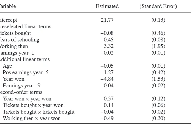
The problem now is how to choose among the (K +1)×(K +2) / 2−1 _fi rst- and second- order terms. I select a subset of these terms in a tepwise fashion. Three choices are to be made by the researcher. First, there may be a subset of the covariates that will be included in the linear part of the speci_fi cation, irrespective of their association with the outcome and the treatment indicator. Note that biases from omitting variables comes from both the correlation between the omitted variables and the treatment indi-cator, and the correlation between the omitted variable and the outcome, just as in the conventional omitted variable formula for regression. In applications to job training programs, these might include lagged outcomes or other covariates that are a priori expected to be substantially correlated with the outcomes of interest. Let us denote this subvector by X_B, with dimension 1≤ KB≤ K +1 (XB always includes the intercept). This vector need not include any covariates beyond the intercept if the researcher has no strong views regarding the relative importance of any of the covariates. Second, a threshold value for inclusion of linear terms has to be speci_fi ed. The decision to in-clude an additional linear term is based on a likelihood ratio test statistic for the null hypothesis that the coef_fi cient on the additional covariate is equal to zero. The thresh-old value will be denoted by C_lin, with the value used in the applications being C_lin = 1. Finally, a threshold value for inclusion of second- order terms has to be speci_fi ed. Again, the decision is based on the likelihood ratio statistic for the test of the null hy-pothesis that the additional second- order term has a coef_fi cient equal to zero. The threshold value will be denoted by C_qua, and the value used in the applications in the current paper is C_qua = 2.71. The values for C_lin and C_qua have been tried out in simula-tions, but there are no formal results demonstrating that these are superior to other values. More research regarding these choices would be useful.

C. Blocking with Regression

[0,1] into J intervals of the form [b_j–1,b_j), for j = 1, . . . , J, where b₀ = 0 and b_J = 1. Let Bi(j)∈{0,1} be a binary indicator for the event that the estimated propensity score for unit i, e(ˆ Xi), satisfi es bj−1<e(Xˆ i)≤bj. Within each block, the average treatment effect is estimated using linear regression with some of the covariates, including an indicator for the treatment

( ˆ␣_j, ˆ␶_j, ˆ␤_j)=arg min ␣,␶,␤ Bi

i=1

N

∑

(j)⋅(Yi−␣−␶⋅Wi− ′␤Xi)

2_.

The covariates included beyond the intercept may consist of all or a subset of the co-variates viewed as most important. Because the coco-variates are approximately balanced within the blocks, the regression does not rely heavily on extrapolation as it might do if applied to the full sample. This leads to J estimates ␶ˆ_j, one for each stratum or block. These J within- block estimates ␶ˆ_j are then averaged over the J blocks, using either the proportion of units in each block, (N_cj + N_tj)/N, or the proportion of treated units in each block, N_tj / N_t, as the weights:

(14) ␶_block(Y,W,X)= Ncj+Ntj N j=1

J

∑

⋅␶ˆ_j, and ␶_block,treat(Y,W,X)= Ntj Nt j=1

J

∑

⋅␶ˆ_j.

The only decision the researcher has to make in order to implement this estimator is the number of blocks, J, and boundary values for the blocks, b_j, for j = 1, . . . , J – 1. Following analytic result by Cochran (1968) for the case with a single normally dis-tributed covariate, researchers have often used _fi ve blocks, with an equal number of units in each block. Here I use a data- dependent procedure for selecting both the number of blocks and their boundaries that leads to a number of blocks that increases with the sample size, developed in Imbens and Rubin (2015).

The algorithm proposed in Imbens and Rubin (2015) relies on comparing average values of the log odds ratios by treatment status, where the estimated log odds ratio is

ˆ

C(x)=ln e(x)ˆ 1−e(x)ˆ ⎛

⎝⎜ ⎞⎠⎟.

Start with a single block, J = 1. Check whether the current strati_fi cation or blocking is adequate. This check is based on the comparison of three statistics, one regarding the correlation of the log odds ratio with the treatment indicator within the current blocks, and two concerning the block sizes if one were to split them further. Calculate the t- statistic for the test of the null hypothesis that the average value for the estimated propensity score for the treated units is the same as the average value for the estimated propensity score for the control units in the block. Speci_fi cally, if one looks at block j, with B_ij = 1 if unit i is in block j (or bj−1≤ e(Xˆ i)<bj), the t- statistic is

t = Ctjˆ −Ccjˆ S_C,j,t

2 _{/ N}

tj+SC,j,c

2 _/N

cj ,

where

ˆ Ccj = 1

Ncj

(1−Wi) i=1

N

∑

⋅Bi(j)⋅C(Xˆ i), ˆCtj = 1 Ntj

Wi i=1

N

S_Ccj 2

= 1

Ncj−1

(1−Wi) i=1

N

∑

⋅Bij⋅( ˆC(Xi)−Ccjˆ ) 2_,

and

S_C2tj = 1 Ntj−1

Wi i=1

N

∑

⋅Bi(j)⋅( ˆC(Xi)−Ctjˆ )2.

If the block were to be split, it would be split at the median of the values of the estimated propensity score within the block (or at the median value of the estimated propensity score among the treated if the focus is on the average value for the treated). For block , denote this median by b_{j–1, j}, and de_fi ne

N₋,c,j= 1_bj−1≤e(ˆ_Xi)<bj−1,j i:_Wi

∑

=0

, N₋,t,j= 1_bj−1≤ˆe(_Xi)<bj−1,j i:_Wi

∑

=1

,

N₊,c,j = 1_bj−1,j≤e(ˆ_Xi)<bj i:_Wi

∑

=0

and N₊,t,j = 1_bj−1,j≤e(ˆ_Xi)<bj i:_Wi

∑

=1

.

The current block will be viewed as adequate if either the t- statistic is suf_fi ciently small (less than tblock

max_{), or if splitting the block would lead to too small a number of}

units in one of the treatment arms or in one of the new blocks. Formally, the current block will be viewed as adequate if either

t ≤tblock max

=1.96,

or

min(N₋,c,j,N−,t,j,N+,c,j,N+,t,j)≤3,

or

min(N₋,c,j+ N−,t,j,N+,c,j+N+,t,j)≤ K +2,

where K is the number of covariates. If all the current blocks are deemed adequate, the blocking algorithm is _fi nished. If at least one of the blocks is viewed as not adequate, it is split by the median (or at the median value of the estimated propensity score among the treated if the focus is on the average value for the treated). For the new set of blocks, the adequacy is calculated for each block, and this procedure continues until all blocks are viewed as adequate.

D. Matching with Replacement and Bias- Adjustment

In this section, I discuss the second general estimation procedure: matching. For gen-eral discussions of matching methods, see Rosenbaum (1989); Rubin (1973a, 1979); Rubin and Thomas (1992ab); Sekhon (2009); and Hainmueller (2012). Here, I discuss a speci_fi c procedure developed by Abadie and Imbens (2006).4 _{This estimator consists} of two steps. First, all units are matched, both treated and controls. The matching is with replacement, so the order in which the units are matched does not matter. After

matching all units, or all treated units if the focus is on the average effect for the treated, some of the remaining bias is removed through regression on a subset of the covariates, with the subvector denoted by Z_i.

For ease of exposition, we focus on the case with a single match. The methods gen-eralize in a straightforward manner to the case with multiple matches. See Abadie and Imbens (2006) for details. Let the distance between two values of the covariate vector

x and x′ be based on the Mahalanobis metric x,x′ =(x− ′x) ˆ′⍀−_X1_{(x− ′x), where ⍀ˆ}

X

is the sample covariance matrix of the covariates. Now for each i, for i = 1, . . . , N, let

m(i) be the index for the closest match, de_fi ned as

m(i)=arg min

j:_{W j}≠_Wi Xi−Xj,

where we ignore the possibility of ties. Given the C(i), de_fi ne

ˆ

Yi(0)=

Yiobs if Wi=0

Ym(i)

obs _{if W}

i=1

⎧ ⎨ ⎪ ⎩⎪

ˆ

Yi(1)=

Ymobs(i), if Wi=0

Yi

obs _ifW

i =1.

⎧ ⎨ ⎪ ⎩⎪ De_fi ne also the matched values for the covariates

ˆ

Xi(0)=

Xi ifWi =0,

Xm(i), ifWi =1,

⎧ ⎨ ⎪ ⎩⎪

ˆ

Xi(1)=

Xm(i), ifWi =0 ,

Xi if Wi=1.

⎧ ⎨ ⎪ ⎩⎪

This leads to a matched sample with N pairs. Note that the same units may be used as a match more than once because we match with replacement. The simple matching estimator discussed in Abadie and Imbens (2006) is ˆ␶_sm =⌺_i=N_{1( ˆY}

i(1)−Yˆi(0)) / N.

Aba-die and Imbens (2006, 2010) suggest improving the bias properties of this simple matching estimator by using linear regression to remove biases associated with differ-ences between Xˆi(0) and Xˆi(1). See also Quade (1982) and Rubin (1973b). First, run

the two least squares regressions

ˆ

Yi(0)=␣c+␤c′Xˆi(0)+␧ci, and ˆYi(1)=␣t+␤t′Xˆi(1)+␧ti,

in both cases on N units, to get the least squares estimates ␤ˆ_c and ␤ˆ_t. Now, adjust the imputed potential outcomes as

ˆ

Yi adj₍₀₎

=

Yi

obs _{, if W}

i= 0

ˆ

Yi(0)+␤ˆ′c(XiXC(i)) , if Wi=1,

⎧ ⎨ ⎪ ⎩⎪ and ˆ

Yiadj(1)=

ˆ

Yi(1)+␤ˆ′t(XiXC(i)) , if Wi= 0

Yi

obs _{, if W}

i=1.

⎧ ⎨ ⎪ ⎩⎪

Now the bias- adjusted matching estimator is

␶_match= 1

N ( ˆYi

adj₍₁₎−_Yˆ i

adj₍₀₎₎

i=1

N

∑

␶_match= 1

Nt

( ˆYi

adj_(1)−Yˆ i

adj₍₀₎₎ i:

∑

_Wi=1

.

In practice, the linear regression bias- adjustment eliminates a large part of the bias that remains after the simple matching. Note that the linear regression used here is very different from linear regression in the full sample. Because the matching ensures that the covariates are well- balanced in the matched sample, linear regression does not rely much on extrapolation the way it may in the full sample if the covariate distribu-tions are substantially different.

E. A General Variance Estimator

In this section, I will discuss an estimator for the variance of the two estimators for average treatment effects. Note that the bootstrap is not valid in general because matching estima-tors are not asymptotically linear. See Abadie and Imbens (2008) for detailed discussions.

1. The weighted average outcome representation of estimators and asymptotic linearity

The fi rst key insight is that most estimators for average treatment effects share a mon structure. This common structure is useful for understanding some of the com-monalities of and differences between the estimators. These estimators, including the blocking and matching estimators discussed in Sections III and IV, can be written as a weighted average of observed outcomes,

ˆ ␶ = 1

Nt

␭_i⋅Yi obs₋ 1

Nc i:_Wi

∑

=1

␭_i⋅Yi obs i:

∑

_Wi=1 with

1 Nt

␭_i=1

i:

∑

_Wi=1

, and 1 Nc

␭_{i =}1

i:_Wi

∑

=0 .

Moreover, the weights ␭_i do not depend on the outcomes Yobs_{, only on the covariates X} and the treatment indicators W. The speci_fi c functional form of the dependence of the weights ␭_i on the covariates and treatment indicators depends on the particular estima-tor, whether linear regression, matching, weighting, blocking, or some combination thereof. Given the choice of the estimator, and given values for W and X, the weights can be calculated. See Appendix B for the results for some common estimators.

2. The conditional variance

Here, I focus on estimation of the variance of estimators for average treatment ef-fects, conditional on the covariates X and the treatment indicators W. I exploit the weighted linear average characterization of the estimators in Equation 17. Hence, the conditional variance is

⺦(ˆ␶|X_,W₎₌ Wi

Nt2

+1−Wi

Nc2

⎛

⎝⎜ ⎞⎠⎟⋅␭i2⋅␴_Wi2(Xi) i=1

N

The only unknown components of this variance are ␴ Wi

2_(X

i). Rather than estimating these conditional variances through nonparametric regression following Abadie and Imbens (2006), I suggest using matching. Suppose unit i is a treated unit. Then, _fi nd the closest match within the set of all other treated units in terms of the covariates. Ignoring ties, let h(i) be the index of the unit with the same treatment indicator as i

closest to X_i:

h(i)=arg min

j=1,...,N,j≠i,_{W j}=Wi Xi− Xj.

Because Xi ≈ Xh(i), and thus ␮1(Xi)≈␮1(Xh(i)), it follows that one can approximate

the difference Y_i – Y_h(i) by

(18) Yi−Yh(i) ≈(Yi(1)−␮1(Xi))+(Yh(i)(1)−␮1(Xh(i))).

The righthand side of Equation 18 has expectation zero and variance equal to ␴₁2_(X

i)+␴1 2_(X

h(i)) ≈2␴1 2_(X

i). This motivates estimating ␴_Wi

2_(X

i) by

ˆ

␴ Wi

2_(X

i)=

1 2(Yi

obs_−Y h(i)

obs₎2_.

Note that this estimator ␴ˆ

Wi

2_(X

i) is not a consistent estimator for ␴_Wi

2_(X

i). However, this is not important because one is interested not in the variances at speci_fi c points in the covariates distribution but, rather, in the variance of the average treatment effect. Following the procedure introduce above, this variance is estimated as:

ˆ

⺦(ˆ␶|X_,W₎₌ Wi

Nt2

+1−Wi

Nc2 ⎛

⎝⎜ ⎞⎠⎟⋅␭i2⋅␴ˆ_Wi2(Xi) i=1

N

∑

.

In principle, one can generalize this variance estimator using the nearest L matches rather than just using a single match. In practice, there is little evidence that this would make much of a difference. Hanson and Sunderam (2012) discusses extensions to clustered sampling.

F. Design: Ensuring Overlap

In this section, I discuss two methods for constructing a subsample of the original data set that is more balanced in the covariates. Both take as input the vector of assignments W and the matrix of covariates X, and select a set of units, a subset of the set of indices {1, 2, . . . , N}, with NT _{elements, leading to a trimmed sample with assignment vector}

WT_{, covariates X}T_{, and outcomes Y}T_{. The units corresponding to these indices will then} be used to apply the estimators for average treatment effects discussed in Sections III and IV.

The _fi rst method is aimed at settings with a large number of controls relative to the number of treated units, and the focus is on the average effect of the treated. This method constructs a matched sample where each treated unit is matched to a distinct control unit. This creates a sample of size 2⋅Nt distinct units, half of them treated and half of them control units. This sample can then be used in the analyses of Sections III and IV.

with the opposite treatment. Their presence makes analyses sensitive to minor changes in the speci_fi cation to the presence of outliers in terms of outcome values. In addition, their presence increases the variance of many of the estimators. The threshold at which units are dropped is based on a variance criterion, following CHIM.

1. Matching without replacement on the propensity score to create a balanced sample

The _fi rst method creates balance by matching on the propensity score. Here we match without replacement. Starting with the full sample with N units, N_t treated and N_c >

N_t controls, the _fi rst step is to estimate the propensity score using the methods from Section II. I then transform this to the log odds ratio,

ˆ

C(x;W_,X_{)= ln} eˆ(x;W,X) 1−eˆ₍x_;W_,X₎

⎛

⎝⎜ ⎞⎠⎟.

To simplify notation, I will drop the dependence of the estimated log odds ratio on X and W and simply write _Cˆ₍x). Given the estimated log odds ratio, the N_t treated obser-vations are ordered, with the treated unit with the highest value of the estimated log odds ratio scored _fi rst. Then, the _fi rst treated unit (the one with the highest value of the estimated log odds ratio) is matched with the control unit with the closest value of the estimated log odds ratio.

Formally, if the treated units are indexed by i = 1, . . . , N_t, with Cˆ(X_i)≥Cˆ(X_i+1), the index of the matched control j(1) satis_fi es W_j(1) = 0, and

j(1)=arg min

i:_Wi=0| ˆ

ˆ

C(X_i)−Cˆ(X₁)|.

Next, the second treated unit is matched to unit j(2), where W_j(2) = 0, and j(2) =arg min

i:_Wi=0,i≠j(1)| ˆC(Xi)−

ˆ

C(X2)|.

Continuing this for all N_t treated units leads to a sample of 2⋅N_t distinct units, half of them treated and half of them controls. Although before the matching the average value of the propensity score among the treated units must be at least as large as the average value of the propensity score among the control units, this need not be the case for the matched samples.

I do not recommend simply estimating the average treatment effect for the treated by differencing average outcomes in the two treatment groups in this sample. Rather, this sample is used as a trimmed sample, with possibly still a fair amount of bias remaining but one that is more balanced in the covariates than the original full sample. As a result, it is more likely to lead to credible and robust estimates. One may augment this procedure by dropping units for which the match quality is particularly poor, say dropping units where the absolute value of the difference in the log odds ratio between the unit and its match is larger than some threshold.

2. Dropping observations with extreme values of the propensity score

covariate space. Let _⺨ be the covariate space and _⺑⊂ _⺨ be some subset of the covariate space. Then de_fi ne ␶(⺑)=⺕[Yi(1)−Yi(0)|Xi∈⺑]. The idea in CHIM is to choose a set ⺑ such that there is substantial overlap between the covariate distributions for treated and control units within this subset of the covariate space. That is, one wishes to exclude from the set _⺑, values for the covariates for which there are few treated units compared the number of control units or vice versa. The question is how to operationalize this. CHIM suggests looking at the asymptotic ef_fi ciency bound for the ef_fi cient estimator for ␶(⺑). The motivation for that criterion is as follows. If there is a value for the covariate such that there are few treated units relative to the number of control units, then for this value of the covariate, the variance for an estimator for the average treatment effect will be large. Excluding units with such covariate values should therefore improve the asymptotic vari-ance of the ef_fi cient estimator. It turns out that this is a feasible criterion that leads to a relatively simple rule for trimming the sample. The trimming also improves the robust-ness properties of the estimators. The trimmed units tend to be units with high leverage whose presence makes estimators sensitive to outliers in terms of outcome values.

CHIM calculates the ef_fi ciency bound for ␶(⺑), building on the work by Hahn (1998), assuming homoskedasticity so that ␴2

=␴₀2_(x)

= ␴₁2_{(x) for all x and a constant} treatment effect, as

␴2 q(⺑)⋅⺕

1

e(X)+ 1

1−e(x) X ∈⺑

⎡ ⎣⎢

⎤ ⎦⎥,

where q(⺑)=Pr(X ∈⺑). It derives the characterization for the set _⺑ that minimizes the asymptotic variance and shows that it has the simple form

(19) ⺑*

={x ∈⺨|␣ ≤e(X)≤1−␣}, where _␣ satis_fi es

1

␣⋅(1−␣) = 2⋅⺕

1

e(X)⋅(1−e(X))

1

e(X)⋅(1−e(X)) ≤ 1

␣⋅(1−␣)

⎡ ⎣⎢

⎤ ⎦⎥.

Crump et al. (2008a) then suggests dropping units with Xi∉⺑

*_{. Note that this}

subsample is selected solely on the basis of the joint distribution of the treatment indi-cators and the covariates and therefore does not introduce biases associated with selec-tion based on the outcomes.

Implementing the CHIM suggestion is straightforward once one has estimated the propensity score. De_fi ne the function g :⺨ 8⺢ with

g(x)= 1

ˆ

e(x)⋅(1−eˆ(x)),

and the function h:⺢ 8⺢ with h(␭)= 1

(⌺_iN₌₁

1{g(_Xi)≤␭})2

1{g(_Xi)≤␭} i=1

N

∑

⋅g(Xi),

one can simply evaluate the function at ␭= g(Xi) for i = 1, . . . , N and select the one

that minimizes h(␭).

The simulations reported in CHIM suggest that, in many settings, in practice the choice _␣ =0.1 leading to

⺑={x∈⺨|0.1≤e(X)≤0.9}

provides a good approximation to the optimal _⺑*_.

G. Assessing Unconfoundedness

Although the unconfoundedness assumption is not testable, the researcher can often do calculations to assess the plausibility of this critical assumption. These calcula-tions focus on estimating the causal effect of the treatment on a pseudo- outcome, a variable known to be unaffected by it, typically because its value is determined prior to the treatment itself. Such a variable can be time- invariant, but the most interesting case is in considering the treatment effect on a lagged outcome, commonly observed in evaluations of labor market programs. If the estimated effect differs from zero, it is less plausible that the unconfoundedness assumption holds, and if the treatment effect on the pseudo- outcome is estimated to be close to zero, it is more plausible that the un-confoundedness assumption holds. Of course, this does not directly test this assump-tion; in this setting, being able to reject the null of no effect does not directly re_fl ect on the hypothesis of interest, unconfoundedness. Nevertheless, if the variables used in this proxy test are closely related to the outcome of interest, the test arguably has more power. For these tests, it is clearly helpful to have a number of lagged outcomes. To formalize this, suppose the covariates consist of a number of lagged outcomes

Y_i,–1, . . . , Y_i,–T as well as time- invariant individual characteristics Z_i, so that the full set of covariates is X_i = (Y_i,–1, . . . , Y_i,–T, Z_i). By construction, only units in the treatment group after period –1 receive the treatment; all other observed outcomes are control outcomes. Also, sup