Automatic Segmentation
of Impaired Joint Space Area
for Osteoarthritis Knee on X-ray Image
using Gabor Filter Based Morphology Process
Lilik Anifah1,I Ketut Eddy Purnama2,Moch. Hariadi2, and Mauridhi Hery Purnomo2
AbstractSegmentation is the first step in osteoarthritis classification. Manual selection is time-consuming, tedious, and expensive. The system is designed to help medical doctors to determine the region of interest of visual characteristics found in knee Osteoarthritis (OA). We propose a fully automatic method without human interaction to segment Junction Space Area (JSA) for OA classification on impaired x-ray image. In this proposed system, right and left knee detection is performed using using Contrast-Limited Adaptive Histogram Equalization (CLAHE) and template macthing. The row sum graph and moment methods are used to segment the junction space area of knee. Overall we evaluated 98 kneess of patients. Experimental results demonstrate an accuracy of the system of up to 100% for detection of both left and right knee and for junction space detection an accuracy 84.38% for the right knee and 85.42% for the left. The
second experiment using gabor filter with parameter α=8, θ=0, Ψ=[0 Π/2], γ=0,8 and N=8 and row sum graph give an accuracy 92.63% for the right knee and 87.37% for the left. And the average time needs to process is 65.79 second. For obvious reasons we chose the results of the fourth to segment junction area in both right and the left knee.
Keywordsknee osteoarthritis, segmentation, joint space width, CLAHE, gabor filter
AbstrakSegmentasi image adalah tahap pertama dalam proses klasifikasi osteoarhtritis. Segmentasi manual memerlukan waktu yang lebih banyak serta memerlukan biaya yang lebih mahal. Sistem yang didesain ini diperuntukkan untuk membantu dokter menentukan region of interest pada penyakit osteoarthritis pada bagian lutut. Penelitian ini merekomendasikan metode untuk menentukan Junction Space Area (JSA) tanpa interaksi manusia untuk image x-ray. Kami mengusulkan penggunaan metode Contrast-limited adaptive histogram equalization (CLAHE) dan template matching untuk mensegmentasi kaki kanan dan kiri. Kombinasi metode Row sum graph, moment dan Gabor Kernel digunakan untuk mensegmentasi Junction Space Area (JSA) pada lutut. Seacara keseluruhan kami mengevaluasi 98 lutut pasien. Hasil eksperimen menunjukkan bahwa untuk mendeteksi kaki kanan dan kiri mempunyai akurasi 100%, sedangkan kemampuan untuk mensegmentasi Junction Space Area (JSA) untu kaki kanan dan kiri adalah 84,38% dan 85,42%. Untuk percobaan kedua kami menggunakan kombinasi Row sum graph, moment dan Gabor Kernel dengan nilai parameter α=8, θ=0, Ψ=[0 Π/2], γ=0,8 dan N=8 menghasilkan akurasi 92,63% untuk lutut kanan dan 87,37% untuk lutut kiri. Rata-rata waktu yang diperlukan selama proses adalah 65,79 second.
Kata Kunciknee osteoarthritis, segmentation, joint space width, CLAHE, gabor filter
I.INTRODUCTION7
he number of people with osteoarthritis in Indonesia is very large 17.533.304 in the year 2004 [1]. Osteoarthritis (OA), the most common joint disorder, comprises a heterogeneous group of syndromes that affect all joint tissues, although the articular cartilage and the adjacent bone often show the most prominent changes. OA represents a leading musculoskeletal health and socioeconomic burden for society worldwide, causing progressive and irreversible articular cartilage tissue damage and, finally, the failure of the joint as a whole organ [2-4].
X-ray, Magnetic Resonance Imaging (MRI) and arthroscopy are the methods most widely used to assess the status of osteoarthritic joints [5]. Some cases were measured by osteo CT [6]. However, in Indonesia it is common to use X-ray or Magnetic Resonance Imaging (MRI).
Lilik Anifah is with Department of Electrical Engineering, Universitas Negeri Surabaya, Indonesia. Email: [email protected].
I Ketut Eddy Purnama, Mochamad Hariadi, and Mauridhi Hery Purnomo are with Department of Electrical Engineering, FTI, Institut Teknologi Sepuluh Nopember, Surabaya, 60111, Indonesia. Email: [email protected], [email protected], [email protected].
Segmentation is the first step in osteoarthritis classification. Manual selection is time-consuming, tedious, and expensive. Even if a radiologist expert or highly trained person is available to select regions, high inter- and intra-ob-server variabilities are still possible [7]. Our ultimate goal is to develop a fully automated system for osteoarthritis classification. Detection and segmentation of joint space area is a component of the automated system that is currently developed. In this study, we propose an automated method for segmentation of the impaired joint space area for knee.
Several methods have been applied to segment knee junction space area of radiograph image, e.g., using a
fi d s t of 20 pr -selected images, such that each image
is a 150×150 window of a center of a joint, Finding the joint in a given knee X-ray imag is p rform d by first downscaling the image by a factor 10, and then scanning the image with a 15×15 shifted window. For each position, the Euclidean distances between the 15×15 pixels of the shifted window and each of the 15×15 pre-d fin pre-d joint imag s [8], pre-d v lop pre-d m thopre-d consists of image preprocessing, delineation of cortical bone plates
(active shape model), and location of regions of interest (ROI) [7], ROI detection is performed using edge based segmentation method. The feature to be extracted is the distance between femur and tibia bone by rotated image, array of mean intensity, the parameter rotation, horizontally translated image and vertically translated image [9]. However this method is exactly implemented in X-ray images of healthy knees but not of impaired knees.
We propose a machine vision system for segmentation of joint space area that could be implemented on X-ray images of healthy and impaired knees, using Contrast-Limited Adaptive Histogram Equalization (CLAHE), template matching using Euclidean distance measures, the row-sum graph and center-of-mass computation.
This journal is outlined as follows: In section 2 we briefly describe material and the proposed method. Experimental results and discussions will be presented in section 3, followed by discussions in section 4, conclusions in section 5, and future work in section 6.
II.METHOD
A. Material
We observed 98 x-ray impaired images data obtained from the Osteoarthritis Initiave (OAI) dataset [10]. The
fi d-fl ion kn -rays were acquired with the beam angle at 10 degrees. The anterior wall of the SynaFlexer positioning frame (provided by Synarc) must be in direct contact with the bucky, cassette holder or reclining table top of the radiographic unit such that there is no angle or gap between them. To ensure these requirements, the bucky or cassette holder is lowered so that the center of
th film ill b at th l v l of th participant’s
tibiofemoral joint line. The center line of the positioning frame is set to the center of the bucky or cassette holder [11].
Hardware specification used in this research is Dell Inspiron N3010 with Processor Intel(R) Core(TM) i5 CPU M430 @2,27 GHz installed memory (RAM) 2,00 GB.
B. Method
We divide the experiment into two stages. The first stage to segment the right knee and the left. And the second stage to find the junction space area of the knee.
Digital radiographs were normalized into 2828×2320 image before segmented. To segment the right and the left knee there are 4 experiments. The first experiment uses only center of mass, the second experiment uses only template matching, the third experiment uses CLAHE and template matching, and the fourth experiment combines CLAHE, template matching, and and center of mass calculation.
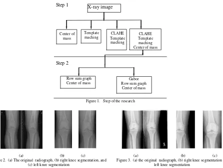
The second stage experiment (the segmentation of junction space area) there are 2 experiments. The first experiment row sum graph and center of mass method and the second experiment uses combine gabor filter, row sum graph and center of mass method. The step of this research is figured in Figure 1.
1. Contrast-limited adaptive histogram equalization Contrast Limited Adaptive Histogram Equalization, CLAHE, is an improved version of AHE, or Adaptive Histogram Equalization. Both overcome the limitations of standard histogram equalization. [12]. CLAHE is a special case of the histogram equalization technique [13]. The procedure of CLAHE technique is described below:
Step 1: Each cell-image was divided into a number of non-overlapping contextual regions of equal sizes, experimentally set to be 2x2, which corresponds to approximately 40 pixels.
Step 2: The histogram of each contextual region was calculated.
Step 3: A clip limit, for clipping histograms, was set (t=0.001). The clip limit was a threshold parameter by which the contrast of the cell-image could be effectively altered; a higher clip limit increased cell-spot contrast.
Step 4: Each histogram was redistributed in such a way that its height did not exceed the clip limit.
Step 5: All histograms were modified by the transformation function is the probability density function of the input image grayscale value j, n is the total number of pixels in the input image and nj is the input pixel number of grayscale value j.
Step 6: The neighboring tiles were combined using bilinear interpolation and the cell-image grayscale values were altered according to the modified histograms [14].
Histogram equalization maps th input imag ’s
intensity values so that the histogram of the resulting image will have an approximately uniform distribution [15].
The histogram of a digital image with gray levels in the range [0, L-1] is a discrete function
p(rk) = nk / n (1) where rk is the kth gray level, nk is the number of pixels in the image with that gray level, n is the total number of pixels in the image, and k =0, 1, 2, …, L-1. Basically p(rk) gives an estimate of the probability of occurrence of gray level rk [16].
2. Template Matching using Euclidean distance
Template Matching is the simplest and the oldest method. It represented by the inner product which is mathematically simple procedure. Template matching can be extended naturally in terms of its mathematical structure to subspace method and also feature matching [17].
Finding position right knee and left knee in a given knee X-ray imag is p rform d by first do nscaling th
2828×2320 image by a factor 30, i.e., x'=round (x/m)
y'=round (y/m) (2)
where m=30 is scale factor, x' is scaled width is y' is scaled height, x is width of the image and y is height of the image.
For right knee the scanning proceeds from x'=1 to x'=18 and y'=1 to y'=20 and left knee the scanning goes from x'=47 to x'=64 and y'=1 to y'=20. Each position the Euclidean distances between the 30×57 pixels are computed as
2 , ' ',
,w ( x y xy)
i I W
d
(3)image I, and di,w is the Euclidean distance between the joint image I and the 30×57 shifted window W.
This simple and fast method was able to successfully find the position right knee and left knee in all images in the dataset. Then we multiply the position with the scale factor.
x = round (x'*m)
y = round (y'*m) (4) After finding the rescaled template position, we
determine its center of mass coordinates
x
c=
M
1,0/
M
0,0andy
c=
M
0,1/
M
0,0withdxdy y x
Mi,j
i j (5)where Mi,j is moment of order i,j. 3. Row sum graph
Once the knees have been located, we use row sum graphs to determine the junction area. The sum graph represents the row-wise summation of the gray values [18]. Let us consider that our input image be F(i, j), the row sum graph S(i, j) is given by
N j j i F j S 1 ) , ( )( (6)
4. Grey level centre of mass
We also determine the center of mass, in terms of gray level in the segmented knee area, to determine the junction area, using the same approach as before, but replacing the binary moment of (7) the gray level counterpart
x y f x ydxdy
Mi,j i j ( , ) (7)
5. Gabor Filter
The formula of complex Gabor function in space domain is given by
g (x,y)=s(x,y)wr(x,y) (8) where s(x,y) is a complex sinusoid, known carrier, and wr(x,y) is 2 dimension gaussian-shaped function, known envelope. The complex sinusoid is defined as follows,
j u x vy P y
x
s( , ) exp 2 0 0 (9)
where (u0,v0) and P define the spatial frequency and the phase of the sinusoid respectively.
The gaussian envelope as follows,
2 0 2 2 0 2 ? exp( ) ,( r r
r x y K a x x b y y
w (10)
where K is scales the magnitude of gaussian envelope, (x0,y0) is the peak of the function, a and b are scalling parameter of the gaussian. And the r subscript stand for rotation operator [19].
III.RESULT AND DISCUSSION
At present, we have developed techniques to perform joint space area automated segmentation and calculation which is necessary for osteoarthritis classification. The segmentation algorithm has been successfully implemented.
A. The First Stage: to Segment the Right Knee and the Left
The first experiment uses only center of mass. For right knee the scanning proceeds from x'=1 to x'=1400 and y'=1 to y'=2320 and left knee the scanning goes from
x'=1400 to x'=2828 and y'=1 to y'=2320. We determine its center of mass coordinates
x
c=
M
1,0/
M
0,0 andwith
(11)
where xc is the center of horizontal mass, yc is the center of vertical mass, and Mi,j moment of the image. The successful result figured in Figure 2 and not successful result figured in Figure 3 and Figure 4.
The second experiment uses only template matching. Finding position right knee and left knee in a given the 2828×2320 knee X-ray image. For right knee the scanning proceeds from x'=1 to x'=1920 and y'=1 to y'=600 and left knee the scanning goes from x'=1 to x'=1920 and y'=1 to y'=600. Each position the Euclidean distances between the 900×1710 pixels are computed as
2 , ' ,' ,w x y xy i I Wd (12)
where Wx,y is the intensity of pixel x, y in the shifted window W, Ix',y' is the intensity of pixel x', y' in the image I, and di,w is the Euclidean distance between the joint image I and the 900×1710 shifted window W. Fig 5 is the successful result of this experiment. Figure 6 and 7 are not successful ones.
The third experiment uses CLAHE and template matching. Before segmented, digital radiographs were normalized into 2828×2320 image then preprocessed
using Contrast-Limited Adaptive Histogram
Equalization (CLAHE). CLAHE is a refinement of adaptive histogram equalization [20]. Histogram
qualization maps th input imag ’s int nsity values so that the histogram of the resulting image will have an approximately uniform distribution [21].
The histogram of a digital image with gray levels in the range [0, L-1] is a discrete function
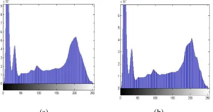
p(rk) = nk / n (13) where rk is the kth gray level, nk is the number of pixels in the image with that gray level, n is the total number of pixels in the image, and k =0, 1, 2, …, L-1. Basically p(rk) gives an estimate of the probability of occurrence of gray level rk. Figure 8 shows the example of original radiograph and the result of preprocessing and Figure 9 is the histogram of the example of original radiograph and the result of preprocessing. Figure 10 is the successful result and Figure 11 is not successful one.
The fourth experiment combines CLAHE, template matching, and center of mass calculation. Finding position right knee and left knee in a given knee X-ray
imag is p rform d by first do nscaling th 2828×2320
image by a factor 30, i.e., x'=round (x/m)
y'=round (y/m) (14) where m=30 is scale factor, x' is scaled width is y' is scaled height, x is width of the image and y is height of the image. We then scan the image with a 30×57 shifted window shown in Figure 12.
For right knee the scanning proceeds from x'=1 to x'=18 and y'=1 to y'=20 and left knee the scanning goes from x'=47 to x'=64 and y'=1 to y'=20. Each position the Euclidean distances between the 30×57 pixels are computed as:
2 , ' , ',w x y xy
i I W
d (15)
image I, and di,w is the Euclidean distance between the joint image I and the 30×57 shifted window W.
This simple and fast method was able to successfully find the position right knee and left knee in all images in the dataset. Then we multiply the position with the scale factor.
x = round(x'*m)
y = round(y'*m) (16) After finding the rescaled template position, we
determine its center of mass coordinates
x
c=
M
1,0/
M
0,0andy
c=
M
0,1/
M
0,0with.dxdy y x
Mi,j
i j (17)where Mi,j is moment of order i,j. The result of the segmentation is shown in Figure 13. Fig (a) is the segmentation of right knee and (b) is the left knee. B. The Second Stage Experiment (the Segmentation of
Junction Space Area)
Once the knees have been located, we use row sum graphs to determine the junction area. The sum graph represents the row-wise summation of the gray values [16]. Let us consider that our input image be F(i,j), the row sum graph S(i j) is given by
N j j i F j S 1 ) , ( )( (18)
Figure 14(a) shows the row sum graph of the right knee and Figure 15(a) the row sum graph of the left knee. The minimum of the graph is the junction space area of knee.
We also determine the center of mass, in terms of gray level in the segmented knee area, to determine the junction area, using the same approach as before, but replacing the binary moment of (5) the gray level counterpart
x y f x ydxdy Mi,j i j ( , )
(19) Figure 14(c) is the result of right knee junction space area segmentation Figure 15(c) is the result of right knee junction space area segmentation.
The formula of complex Gabor function in space domain is given by
g (x,y)=s(x,y)wr(x,y) (20)
where s(x,y) is a complex sinusoid, known carrier, and wr(x,y) is 2 dimension gaussian-shaped function, known envelope. The complex sinusoid is defined as follows,
j u x v y P y
x
s( , ) exp 2 0 0 (21) where (u0,v0) and P define the spatial frequency and the phase of the sinusoid respectively.
The gaussian envelope as follows,
2 0 2 2 0 2 ? exp( ) ,( r r
r x y K a x x b y y
w (22)
where K is scales the magnitude of gaussian envelope, (x0,y0) is the peak of the function, a and b are scalling parameter of the gaussian. r subscript stand for rotation operator [17].
At present, we have developed techniques to perform joint space area automated segmentation and calculation which is necessary for osteoarthritis classification. The segmentation algorithm has been successfully implemented. The system's accuracy of each stage is shown in Table 1.
Experiment 4 give accuracy 100% for both knee
because it used combine techniques used Experiment 1, 2 and 3. The first experiment uses only center of mass, it give 95.83% for right knee and 86.46% for the left. The second experiment uses only template matching give accuracy 83.33% and 60.43%, limitation of this method in some cases the region of interest could be twist. The third experiment uses CLAHE and template matching give accuracy 89.58% and 83.33% for the left, weakness of this experiment are the speed and some cases the region of interest still could be twist although the intensity had normalized by CLAHE. Fourth experiment combines CLAHE, template matching, and center of mass calculation for finding position right knee and left knee using downscalling method. CLAHE used for normalized the intensity, template matching used for finding the region of interest, and center of mass is solution to minimize possibility twist between the right and the left. The fourth experiment give accuracy 100% for both knee. Speed is faster then experiment 1, 2, 1nd 3 because for finding position right knee and left knee using downscalling the 2828×2320 image by a factor 30. After finding the position, we multiply the position with the scale factor then we determine its center of mass coordinates.
The second stage experiment (the segmentation of junction space area) using row sum graph and center of mass method give an accuracy 84.38% for the right knee and 85.42% for the left. And the average time needs to process is 1.404 second. The second experiment using gabor filt r ith param t r α=8, θ=0, ψ=[0 π/2], γ=0,8 and n=8 and row sum graph give an accuracy 92.63% for the right knee and 87.37% for the left. And the average time needs to process is 65.79 second. For accuracy and speed reasons we chose the results of the fourth to segment junction area in both right and the left knee.
Segmentation is the first step in osteoarthritis classification. We propose a fully automatic method to segment junction space area for OA classification on impaired x-ray image. Future plans we develop fully automatic technique to classify knee X-rays using expert system.
IV.CONCLUSION
In this reearch, the proposed technique is an effective junction space area segmentation method without the need for user interaction. Experimental results have been provided to show the effectiveness of the proposed technique. And could help medical doctors to determine the region of interest of visual characteristics found in knee OA. The failures in junction detection may well be due to deviations of the angle of the knee joint from the horizontal. We will improve this by including gradient information in the junction area segmentation.
ACKNOWLEDGMENT
Figure 1. Step of the research
(a) (b) (c)
Figure 2. (a) The original radiograph, (b) right knee segmentation, and (c) left knee segmentation
(a) (b) (c)
Figure 3. (a) the original radiograph, (b) right knee segmentation (c) left knee segmentation
(a) (b) (c)
Figure 4. (a) the original radiograph (b) right knee segmentation (c) left knee segmentation
(a) (b) (c)
Figure 5. (a) the original radiograph (b) right knee segmentation (c) left knee segmentation
(a) (b) (c)
Figure 6. (a) the original radiograph (b) right knee segmentation (c) left knee segmentation
(a) (b) (c)
Figure 7. (a) the original radiograph (b) right knee segmentation (c) left knee segmentation
X-ray image
Center of mass
Template
maching Template CLAHE maching
CLAHE Template maching Center of mass Step 1
Step 2
Row sum graph
(a) (b)
Figure 8. Comparison of (a) the original radiograph and (b) the result of the processing
(a) (b)
Figure 9. Comparison (a) histogram of the original radiograph and (b) histogram of the result of the processing
(a) (b) (c)
Figure 10. (a) preprocessed image (b) right knee segmentation (c) left knee segmentation
(a) (b) (c)
Figure 11. (a) preprocessed image (b) right knee segmentation (c) left knee segmentation
(a) (b)
Fig 12. A 30×57 shifted window used for finding the position of (a) left knee (b) right knee
(a) (b)
Figure 13. Segmentation Result (a) right knee and and (b) left knee
(a) (b) (c)
Figure 14. (a) Row sum graph of right knee (b) right knee (c) junction space area of right knee
(a) (b) (c) Figure 15. (a) Row sum graph of left knee (b) left knee and (c)
junction space area of left knee
TABLE 1.
SYSTEM'S ACCURACY OF EACH STAGE
Experiment Accuracy (Seconds) Time
Right Knee (%) Left Knee (%)
1 95,83 86,46 0,82
2 83,33 60,42 0,8745
3 89,58 83,33 0,91
REFERENCES
[1] http://www.wrongdiagnosis.com/o/osteoarthritis/stats-country.html [2] A. D. Woolf and B. Pfl g r “Burd n of major musculosk l tal conditions”, Bull World Health Organ, vol. 81, pp. 646-656, 2003.
[3] M. J. Elders, “The increasing impact of arthritis on public health,”
Journal Rheumatol, vol. 60, pp. 6-8, 2000.
[4] J. Martel-Pelletier, D. Lajeunesse, H. Fahmi, G. Tardif, and J. P. Pelletier ,“New thoughts on the pathophysiology of osteoarthritis: one more step toward new therapeutic targets,” Curr Rheumatol
Rep, vol. 8, pp. 30-6, 2006.
[5] Buckland-Wright, “Current status of imaging procedures in the diagnosis, prognosis and monitoring of osteoarthritis,” Bailliere's Clinical Rheumatology, vol. 11, no. 4, Nov. 1997.
[6] El Miedany, “Altered bone mineral metabolism in patients with osteoarthritis, Éditions sci ntifiqu s t médical s Els vi r SAS, 67 : 521-7, 2000.
[7] P. Podsiadlo, M. Wolski, and G. W. Stacho iak, “Automat d s l ction of trab cular bon r gions in kn radiographs”, Medical Physics, vol. 35, no. 5, pp. 1870-1882, May 2008.
[8] L. Shamir, S. M. Ling, W. W. Scott, A. Bos, and N. Orlov, “Kn X-ray image analysis method for automated detection of Osteoarthritis,” IEEE Transactions on Biomedical Engineering, 2008, pp. 1-10.
[9] T. L. Mengko, R. G. Wachjudi, A. B. Suksmono, and Q. Danudirdjo, “Automat d D tection of Unimpaired joint space for knee osteoarthritis assessment”, 0-7803 -8940-9/050 IEEE, pp. 400-403, 2005.
[10] http://oai.epi-ucsf.org/datarelease/
[11] Ost oarthritis Initiativ : A Kn H alth Study, “ adiographic Procedure Manual for Examinations of the Knee, Hand, Pelvis and Lo r Limbs”, OAI, San Frasisco, 2006.
[12] http://radonc.ucsf.edu/research_group/jpouliot/tutorial/HU/Lesson 7.html
[13] R.C. Gonzalez and R.E. Woods, Digital image processing, 1992.
[14] D. Cavouras, “An Efficient Clahe-Based, Spot-Adaptive, Image S gm ntation T chniqu for Improving Microarray G n s’ Quantification,” presented at 2nd International Conference on
Experiments /Process/System Modelling/Simulation & Optimization 2nd IC-EpsMsO Athens, 4-7 July, 2007.
[15] J. E. Barn s “Charact ristics and control of contrast in CT. RadioGraphics” vol. 12. 1992, pp. 825-837.
[16] R. C. Gonzalez, R. E. Woods, and S. L. Eddins, Digital image processing using matlab, Pearson Education, 2005.
[17] Mori, Optical Character Recognition, John Willey and Son, Canada, 1999.
[18] M. Mehta and R. Sanchati, and A. Marchya, “Automatic Cheque Processing System,” International Journal of Computer and Electrical Engineering, vol. 2, no. 4, pp. 761-765, August 2010. [19] J. . Mov llan, “Tutorial on Gabor Filt rs”, 2008.
[20] Nixon, Feature Extraction and Image Processing 2nd ed, Elsevier,
2008.