48
In this chapter, the writer would like to discuss the result of the study which covers the data presentation, the result of data analysis, and discussion.
A. Data Presentation
In this chapter, the writer presented the obtained data. The data were presented in the following steps.
1. Distribution of Pre Test Scores of the Experiment Group
The pre test scores of the experiment group were presented in the following table.
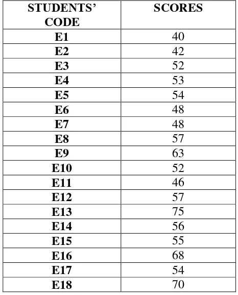
Table 4.1 The Description of Pre Test Scores of The Data Achieved by The Students in Experiment Group
STUDENTS’
CODE
SCORES
E1 40
E2 42
E3 52
E4 53
E5 54
E6 48
E7 48
E8 57
E9 63
E10 52
E11 46
E12 57
E13 75
E14 56
E15 55
E16 68
E17 54
E19 51
E20 70
E21 70
E22 51
E23 53
E24 48
E25 52
E26 60
The Highest Score (H) = 75 The Lowest Score (L) = 40
The Range of Score (R) = H – L + 1 = 75 – 40 + 1 = 36
The Class Interval (K) = 1 + (3.3) x Log n = 1 + (3.3) x Log 26 = 1 + (3.3) x 1.41 = 1 + 4.653 = 5.653 = 6
Interval of Temporary (I) =
=
= 6
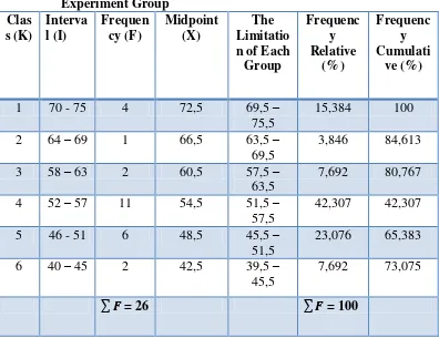
Table 4.2 The Frequency Distribution of the Pre Test Scores of the Experiment Group
0
39.5-45.5 45.5-51.5 51.5-57.5 57.5-63.5 63.5-69.5 69.5-75.5 2 The Frequency Distribution of the Pre Test Scores of
Experiment Group
The table and figure above showed the pre test score of students in experiment group. It could be seen that there were 2 students who got score 39,5-45,5. There were 6 students who got score 45,5-51,5. There were 11 students who got score 51,5-57,5. There were 2 students who got score 57,5-63,5. There was 1 student who got score 63,5-69,5. And there were 4 students who got score 69,5-75,5.
The next step, the writer tabulated the scores into the table for the calculation of mean, median, and modus as follows:
Table 4.3 The Calculation of Mean, Median, and Modus of the Pre Test Scores of the Experiment Group
(I) (F) (X) FX fk (a) fk (b)
70 - 75 4 72,5 290 4 26
64 – 69 1 66,5 66,5 5 22
58 – 63 2 60,5 121 7 21
52 – 57 11 54,5 467,5 18 19
46 - 51 6 48,5 291 24 8
40 – 45 2 42,5 109 26 2
N = 26 ∑ =
1345
a. Mean
Mx = ∑
=
= 51.7 b. Median
= 51.5 +
x
5
= 51.5 +
x 5
= 51.5 + (-0.54) x 5 = 51.5 + (-2.72)
= 48.77
c. Modus
Mo =
+
(
)
= 51.5 +
(
)
x 5= 51.5 +
(
)
x 5= 51.5 + 1.25 = 52.75
The calculation above showed of mean value was 51.7, median value was 48.77, and modus value was 52.75 of the pre test of the experiment group. The last step, the writer tabulated the scores of pre test of experiment group into the table for the calculation of standard deviation and the standard error as follows:
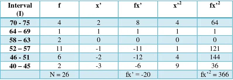
Table 4.4 The Calculation of the Standard Deviation and the Standard Error of the Pre Test Scores of Experimental Group
Interval (I)
f x’ fx’ x’2 fx’2
70 - 75 4 2 8 4 64
64 – 69 1 1 1 1 1
58 – 63 2 0 0 0 0
52 – 57 11 -1 -11 1 121
46 - 51 6 -2 -12 4 144
40 – 45 2 -3 -6 9 36
a. Standard Deviation
b. Standard Error
1
2. Distribution of Pre Test Scores of the Control Group
The pre test scores of the control group were presented in the following table.
Table 4.5 The Description of Pre Test Scores of The Data Achieved by The Students in Control Group
STUDENTS’ CODE SCORES
C1 80
C2 70
C3 60
C4 70
C5 56
C6 45
C7 65
C8 50
C9 65
C10 44
C11 53
C12 53
C13 42
C14 60
C15 53
C16 60
C17 55
C18 55
C19 42
C20 48
C21 45
C22 80
C23 75
C24 54
C25 40
C26 48
The Highest Score (H) = 80 The Lowest Score (L) = 40
= 41
The Class Interval (K) = 1 + (3.3) x Log n = 1 + (3.3) x Log 26 = 1 + (3.3) x 1.41 = 1 + 4.653 = 5.653 = 6
Interval of Temporary (I) =
=
= 6,833 = 7
So, the range of score was 50, the class interval was 6, and interval of temporary was 8. Then, it was presented using frequency distribution in the following table:
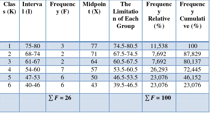
Table 4.6 The Frequency Distribution of the Pre Test Scores of the Control Group
Clas s (K)
Interva l (I)
Frequenc y (F)
Midpoin t (X)
The Limitatio n of Each
Group
Frequenc y Relative
(%)
Frequenc y Cumulati
ve (%)
1 75-80 3 77 74.5-80.5 11,538 100
2 68-74 2 71 67.5-74.5 7,692 87,829
3 61-67 2 64 60.5-67.5 7,692 80,137
4 54-60 7 57 53.5-60.5 26,293 72,445
5 47-53 6 50 46.5-53.5 23,076 46,152
6 40-46 6 43 39.5-46.5 23,076 23,076
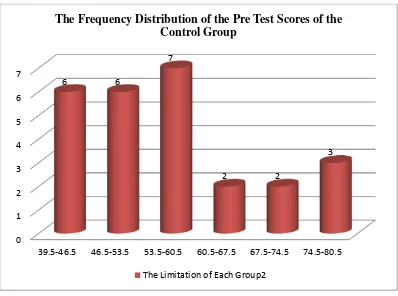
Figure 4.2 The Frequency Distribution of the Pre Test Scores of the Control Group
The table and the figure showed the pre test score of students in control group. It could be seen that there were 6 students who got score 39.5 – 46.5. There were 6 students who got score 46.5 – 53.5. There were 7 students who got score 53.5 – 60.5. There were 2 students who got score 60.5 – 67.5. There were 2 students who got score 67.5 – 74.5 and there were 3 students who got score 74.5 – 80.5.
The next step, the writer tabulated the score into the table for the calculation of mean, median, and modus as follows:
0 1 2 3 4 5 6 7
39.5-46.5 46.5-53.5 53.5-60.5 60.5-67.5 67.5-74.5 74.5-80.5
6 6
7
2 2
3 The Frequency Distribution of the Pre Test Scores of the
Control Group
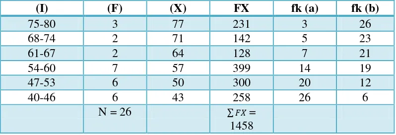
Table 4.7 The Calculation of Mean, Median, and Modus of the Pre Test Scores of the Control Group
(I) (F) (X) FX fk (a) fk (b)
75-80 3 77 231 3 26
68-74 2 71 142 5 23
61-67 2 64 128 7 21
54-60 7 57 399 14 19
47-53 6 50 300 20 12
40-46 6 43 258 26 6
N = 26 ∑ =
1458
a. Mean
Mx = ∑
=
= 56.076 b. Median
Mdn =
= 53.5 +
x
7= 53.5 + x 7
= 53.5 + 0.142 x 7 = 53.5 + 1
= 54.5 c. Modus
Mo =
+
(
= 53.5 +
(
)
x 7= 53.5 +
(
)
x 7= 53.5 + 0.25 x 7 = 55.25
The calculation above showed of mean value was 56.076, median value was 54.5, and modus value was 55.25 of the pre test of the control group.
The last step, the writer tabulated the scores of pre test of control group into the table for the calculation of standard deviation and the standard error as follows:
Table 4.8 The Calculation of the Standard Deviation and the Standard Error of the Pre Test Scores of Control Group
013225
b. Standard Error
1
The result of calculation showed the standard deviation of pre test score of control group was 22.995 and the standard error of pre test score of control group was 4.599.
3. Distribution of Post Test Scores of the Experiment Group
Table 4.9 The Description of Post Test Scores of The Data Achieved by The Students in Experiment Group
STUDENTS’
CODE
SCORES
E1 80
E2 78
E3 65
E4 55
E5 75
E6 83
E7 80
E8 73
E9 78
E10 65
E11 80
E12 63
E13 70
E14 65
E15 57
E16 77
E17 78
E18 65
E19 77
E20 70
E21 76
E22 80
E23 60
E24 75
E25 75
E26 60
The Highest Score (H) = 83 The Lowest Score (L) = 55
The Range of Score (R) = H – L + 1 = 83 – 55 + 1 = 29
= 1 + (3.3) x 1.41 = 1 + 4.653 = 5.653 = 6
Interval of Temporary (I) =
=
= 4,8 = 5
So, the range of score was 36, the class interval was 6, and interval of temporary was 5. Then, it was presented using frequency distribution in the following table:
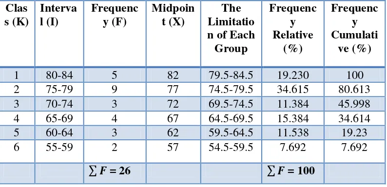
Table 4.10 The Frequency Distribution of the Post Test Score of the Experiment Group
Clas s (K)
Interva l (I)
Frequenc y (F)
Midpoin t (X)
The Limitatio n of Each
Group
Frequenc y Relative
(%)
Frequenc y Cumulati
ve (%)
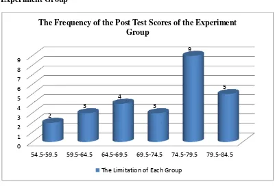
1 80-84 5 82 79.5-84.5 19.230 100
2 75-79 9 77 74.5-79.5 34.615 80.613
3 70-74 3 72 69.5-74.5 11.384 45.998
4 65-69 4 67 64.5-69.5 15.384 34.614
5 60-64 3 62 59.5-64.5 11.538 19.23
6 55-59 2 57 54.5-59.5 7.692 7.692
Figure 4.3 The Frequency Distribution of the Post Test Scores of the Experiment Group
The table and figure above showed the post test score of students in experiment group. It could be seen that there were 2 students who got score 54.5-59.5. There were 3 students who got score 59.5 – 64.5. There were 4 students who got score 64.5 – 69.5. There were 3 students who got 69.5 – 74.5. There were 9 students who got 74.5 – 79.5 and there were 5 students who got 79.5 – 84.5.
The next step, the writer tabulated the score into the table for the calculation of mean, median, and modus as follows:
Table 4.11 The Calculation of Mean, Median, and Modus of the Post Test Scores of the Experiment Group
(I) (F) (X) FX fk (a) fk (b)
80-84 5 82 410 5 26
75-79 9 77 693 14 21
70-74 3 72 216 17 12
65-69 4 67 268 21 9
60-64 3 62 186 24 5
0 1 2 3 4 5 6 7 8 9
54.5-59.5 59.5-64.5 64.5-69.5 69.5-74.5 74.5-79.5 79.5-84.5 2
3
4
3
9
5 The Frequency of the Post Test Scores of the Experiment
Group
55-59 2 57 114 26 2
N = 26 ∑ =
1887 a. Mean
Mx = ∑
=
= 72.576
b. Median
Mdn =
= 74.5 +
x
6= 74.5 + x 6
= 74.5 + 0.1 x 6
= 74.5 + 0.6
= 75.1
c. Modus
Mo =
+
(
= 74.5 +
(
The calculation above showed of mean value was 72.576, median value was 75.1, and modus value was 76.24 of the post test of the experiment group.
The last step, the writer tabulated the scores of post test of the experiment group into the table for the calculation of standard deviation and the standard error as follows:
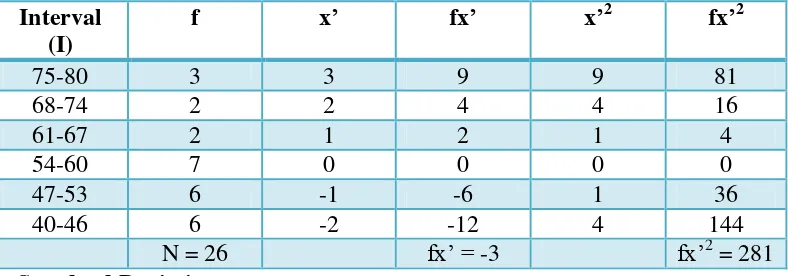
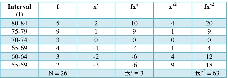
Table 4.12 The Calculation of the Standard Deviation and the Standard Error of the Post Test Scores of Experiment Group
Interval
a. Standard Deviation
013225 b. Standard Error
1
The result of calculation showed the standard deviation of post test score of experiment group was 7.76 and the standard error of post test score of experiment group was 1.552.
4. Distribution of Post Test Scores of the Control Group
Table 4.13 The Description of Post Test Scores of The Data Achieved by The Students in Control Group
STUDENTS’ CODE SCORES
C1 70
C2 65
C3 65
C4 75
C5 66
C6 72
C7 77
C8 71
C9 65
C10 70
C11 73
C12 60
C13 70
C14 84
C15 73
C16 73
C17 70
C18 64
C19 70
C20 77
C21 70
C22 71
C23 65
C24 77
C25 60
C26 75
The Highest Score (H) = 84 The Lowest Score (L) = 60
The Range of Score (R) = H – L + 1 = 84 – 60 + 1 = 25
= 1 + (3.3) x 1.41 = 1 + 4.653 = 5.653 = 6
Interval of Temporary (I) =
=
= 4,167 = 5
So, the range of score was 25, the class interval was 6, and interval of temporary was 5. Then, it was presented using frequency distribution in the following table:
Table 4.14 The Frequency Distribution of the Post Test Scores of the Control Group
Clas s (K)
Interva l (I)
Frequenc y (F)
Midpoin t (X)
The Limitatio n of Each
Group
Frequenc y Relative
(%)
Frequenc y Cumulati
ve (%)
1 80-84 1 82 79.5-84.5 3.846 100
2 76-79 3 77.5 75.5-79.5 11.538 88.458
3 72-75 6 73.5 71.5-75.5 23.076 76.92
4 68-71 8 69.5 67.5-71.5 30.769 53.844
5 64-67 6 65.5 63.5-67.5 23.076 30.768
6 60-63 2 61.5 59.5-63.5 7.692 7.692
Figure 4.4 The Frequency Distribution of the Post Test Scores of the Control Group
The table and the figure showed the post test score of students in control group. It could be seen that there were 2 students who got score 59.5 – 63.5. There were 6 students who got score 63.5 – 67.5. There were 8 students who got score 67.5 – 71.5. There were 6 students who got score 71.5 – 75.5. There were 3 students who got score 75.5 – 79.5 and there was 1 student who got score 79.5 – 84.5.
The next step, the writer tabulated the score into the table for the calculation of mean, median, and modus as follows:
0 1 2 3 4 5 6 7 8
59.5-63.5 63.5-67.5 67.5-71.5 71.5-75.5 75.5-79.5 79.5-84.5 2
6
8
6
3
1 The Frequency Distribution of the Post Test Scores of the
Control Group
Table 4.15 The Table for the Calculation of Mean, Median, and Modus of the Post Test Scores of the Control Group
(I) (F) (X) FX fk (a) fk (b)
80-84 1 82 82 1 26
76-79 3 77.5 232.5 4 25
72-75 6 73.5 441 10 22
68-71 8 69.5 556 18 16
64-67 6 65.5 393 24 8
60-63 2 61.5 123 26 2
N = 26 ∑ =
1827.5
a. Mean
Mx = ∑
=
= 70.288 b. Median
Mdn =
= 67.5 +
x
5= 67.5 + x 5
= 67.5 + 0.83 x 5
= 67.5 + 4.15
c. Modus
Mo =
+
(
)
= 67.5 +
(
)
x 5= 67.5 +
(
)
x 5 = 67.5 + 0.5 x 5 = 67.5 + 2.5 = 70The calculation above showed of mean value was 70.288, median value was 71.65, and modus value was 70 of the post test of the control group.
The last step, the writer tabulated the scores of pre test of control group into the table for the calculation of standard deviation and the standard error as follows:
Table 4.16 The Table of Calculation of the Standard Deviation and the Standard Error of the Post Test Scores of Control Group
Interval (I)
f x’ fx’ x’2 fx’2
80-84 1 3 3 9 9
76-79 3 2 6 4 12
72-75 6 1 6 1 6
68-71 8 0 0 0 0
64-67 6 -1 -6 1 6
60-63 2 -2 -4 4 8
a. Standard Deviation
b. Standard Error
The result of calculation showed the standard deviation of post test score of control group was 6.2 and the standard error of post test score of control group was 1.24.
B. The Result of Data Analysis
1. Testing Hyphothesis Using Manual Calculation and SPSS 16
To test the hypothesis of the study, the writer used t-test statistical calculation. Firstly, the writer calculated the standard deviation and the standard error of X1 and X2. It was found the standard deviation and the standard error of post test of X1 and X2 at the previous data presentation. It could be seen on this following table.
Table 4.17 The Standard Deviation and the Standard Error of X1 and X2
Variables The Standard Deviation The Standard Error
X1 7.76 1.552
X2 6.2 1.24
Where :
X1 = Experiment Group
X2 = Control Group
From the calculation can be seen that :
SEm1– SEm2 = √ +
= √ +
= √
= 1.986
Then, it was inserted to the to formula to get the value of t observe as follows:
o
t
=
2 1
2 1
M
M SE
SE M M
to =
986 . 1
288 . 70 576 . 72
to = 1.986 288 . 2
to = 1.152
With the criteria:
If t-test (t-observed) ≥ ttable,it means Ha is accepted and Ho is rejected.
If t-test (t-observed) < ttable,it means Ha is rejected and Ho is accepted.
df = (N1N2 2)
= (26262) = 50
table
t
at df 50 at 5% significant level = 2.01The calculation above showed the result of t-test calculation as in the table follows:
Table 4.18 The Result of T-test
Variables Tobserved T table Df/Db
5% 1%
X1-X2 1.152 2.01 2.68 50
Where:
X1 = Experimental Group
X2 = Control Group
t observe = The calculated Value
t table = The distribution of t value
df/db = Degree of Freedom
Based on the result of hypothesis test calculation, it was found that the value of tobserved was lower than the value of table at 1% and 5% significance level or 2.01<1.152>2.68. It meant Ha was rejected and Ho was accepted.
non Inductive Method was rejected and Ho stating that the students taught by Inductive Method do not apply better grammar than those taught by non Inductive Method was accepted. Therefore teaching grammar using Inductive Method did not gave significant effect on the students’ grammatical use of the second grade students of MTs. Islamiyah Palangkaraya.
2. Testing Hypothesis Using SPSS Program
The writer used SPSS 19 to measure t-value, the result of t-value in the SPSS would be consulted with t-table in the significance at 5%. Here the computation of t-value using SPSS:
Levene's Test for Equality of
Variances t-test for Equality of Means
F Sig. t df
Sig. (2-tailed)
Mean Differenc
e
Std. Error Difference
95% Confidence Interval of the
Difference Lower Upper Post
Test Scor es
Equal variances assumed
7.976 .007 .636 50 .528 1.231 1.936 -2.658 5.119
Equal variances not assumed
The result of calculation using SPSS 19 program also supported the result of
manual calculation. From the result of t-value using SPSS above was found that H0 was
accepted. It was found tobserved (1.152 or based on SPSS 0.636) was lower than ttable (2,01)
in the significance level of 5%. Even though, the different calculation of t test between
manual calculation and SPSS calculation was 0.516 but it still could be interpreted that
alternative hypothesis (Ha) was rejected. It meant students who are taught by using
Inductive Method did not gave significant effect on the students’ grammatical use
of the second grade students of MTs. Islamiyah Palangkaraya.
3. Testing Normality and Homogenity Using SPSS Program a. Normality
The writer used SPSS 16 to measure the normality of the data as the following below.
One-Sample Kolmogorov-Smirnov Test
Unstandardized
Residual
N 26
Normal Parametersa Mean .0000000
Std. Deviation 8.14756193
Most Extreme Differences Absolute .187
Positive .118
Negative -.187
Kolmogorov-Smirnov Z .955
Asymp. Sig. (2-tailed) .322
The criteria of the normality test of pre-test and post-test is the value of r (probability value/critical value) is higher than or equal to the level of significance alpha defined (r ), it means that the distribution is normal.1 In fact, based on the calculation above the value of r (probability value) from the test in Kolmogorov-Smirnov table was higher than the level of significance alpha used or r was 0,955 higher than 0,05 (∂ value). Thus, the distribution were normal, it meant that the students’ score of the test had normal distribution.
b. Homogeneity
The writer used SPSS 16 to measure the homogeneity of the data as the following below.
Test of Homogeneity of Variance
Levene Statistic df1 df2 Sig.
Post Test Scores Based on
Mean 7.976 1 50 .007
Based on
Median 3.684 1 50 .061
Based on
Median and
with adjusted
df
3.684 1 42.485 .062
Based on
trimmed
mean
7.539 1 50 .008
1
C. Discussion
The result of the analysis shows that Inductive Method did not give significant effect to the students’ grammatical use. It could be proved from the
students’ score; the students taught grammar using Inductive Method reached
almost same score than those who taught without using Inductive Method. It was found the mean of experiment group score (X1) was 72.576 and the mean of control group score (X2) was 70.288. Then, those results were compared using T-test and it was found tobserved computation using manual was 1.152 and ttable was 2, 01. It meant, from the computation was found tobserved > ttable.
Those statistical findings were suitable with the theories as mentioned before in
chapter 2. Actually, the use of this method has been noted for its success in foreign
or second language classroom world-wide. It may help the teacher to vary and organize the lesson, in order to keep classes interesting and motivating for the students. Moreover, learners can improve their learning when they are aware of what they are doing, how they are doing it,and what possibilities are available to them. Inductive method can make grammar lessons enjoyable. They will able to acquire the grammar in an easier manner.2 But, the result of this research showed
that the Inductive Method can not effect the grammar’s score of the students.
There are some reasons why using Inductive Method did not give effect on
the students’ grammar score of the second grade students at MTs. Islamiyah
2
Palangkaraya. Based on the weakness of this method, first, the students can not work out the rules of grammar from the examples by themselves because of their previous method. They were not ready to accept this method. It was in lined with the theory that was mentioned in chapter 2 page 17 about the weakness of inductive method.
Second, Inductive Method was a completely new technique for the students of MTs. Islamiyah Palangkaraya. It was showed from the students’ response that they were not very enthusiastic and are confused when they were taught by using Inductive Method.