CHAPMAN & HALL/CRC
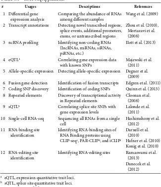
Mathematical and Computational Biology Series
Aims and scope:
This series aims to capture new developments and summarize what is known over the entire spectrum of mathematical and computational biology and medicine. It seeks to encourage the integration of mathematical, statistical, and computational methods into biology by publishing a broad range of textbooks, reference works, and handbooks. The titles included in the series are meant to appeal to students, researchers, and professionals in the mathematical, statistical and computational sciences, fundamental biology and bioengineering, as well as interdisciplinary researchers involved in the field. The inclusion of concrete examples and applications, and programming techniques and examples, is highly encouraged.
Series Editors N. F. Britton
Department of Mathematical Sciences University of Bath
Xihong Lin
Department of Biostatistics Harvard University
Nicola Mulder
University of Cape Town South Africa
Maria Victoria Schneider
European Bioinformatics Institute
Mona Singh
Department of Computer Science Princeton University
Anna Tramontano
Department of Physics
University of Rome La Sapienza
Proposals for the series should be submitted to one of the series editors above or directly to: CRC Press, Taylor & Francis Group
Published Titles
An Introduction to Systems Biology: Design Principles of Biological Circuits Uri Alon
Glycome Informatics: Methods and Applications
Kiyoko F. Aoki-Kinoshita
Computational Systems Biology of Cancer
Emmanuel Barillot, Laurence Calzone, Philippe Hupé, Jean-Philippe Vert, and Andrei Zinovyev
Python for Bioinformatics
Sebastian Bassi
Quantitative Biology: From Molecular to Cellular Systems
Sebastian Bassi
Methods in Medical Informatics: Fundamentals of Healthcare
Programming in Perl, Python, and Ruby
Jules J. Berman
Computational Biology: A Statistical Mechanics Perspective
Ralf Blossey
Game-Theoretical Models in Biology
Mark Broom and Jan Rychtáˇr
Computational and Visualization Techniques for Structural Bioinformatics Using Chimera
Forbes J. Burkowski
Structural Bioinformatics: An Algorithmic Approach
Forbes J. Burkowski
Spatial Ecology
Stephen Cantrell, Chris Cosner, and Shigui Ruan
Cell Mechanics: From Single Scale-Based Models to Multiscale Modeling
Arnaud Chauvière, Luigi Preziosi, and Claude Verdier
Bayesian Phylogenetics: Methods, Algorithms, and Applications
Ming-Hui Chen, Lynn Kuo, and Paul O. Lewis
Statistical Methods for QTL Mapping
Zehua Chen
Normal Mode Analysis: Theory and Applications to Biological and Chemical Systems
Qiang Cui and Ivet Bahar
Kinetic Modelling in Systems Biology
Oleg Demin and Igor Goryanin
Data Analysis Tools for DNA Microarrays
Sorin Draghici
Statistics and Data Analysis for Microarrays Using R and Bioconductor, Second Edition
Sorin Draghici˘
Computational Neuroscience: A Comprehensive Approach Jianfeng Feng
Biological Sequence Analysis Using the SeqAn C++ Library
Andreas Gogol-Döring and Knut Reinert
Gene Expression Studies Using Affymetrix Microarrays
Hinrich Göhlmann and Willem Talloen
Handbook of Hidden Markov Models in Bioinformatics
Martin Gollery
Meta-analysis and Combining Information in Genetics and Genomics
Rudy Guerra and Darlene R. Goldstein
Differential Equations and Mathematical Biology, Second Edition
D.S. Jones, M.J. Plank, and B.D. Sleeman
Knowledge Discovery in Proteomics
Igor Jurisica and Dennis Wigle
Introduction to Proteins: Structure, Function, and Motion
Amit Kessel and Nir Ben-Tal
RNA-seq Data Analysis: A Practical Approach
Eija Korpelainen, Jarno Tuimala,
Panu Somervuo, Mikael Huss, and Garry Wong
Biological Computation
Ehud Lamm and Ron Unger
Optimal Control Applied to Biological Models
Clustering in Bioinformatics and Drug Discovery
John D. MacCuish andNorah E. MacCuish
Spatiotemporal Patterns in Ecology and Epidemiology: Theory, Models, and Simulation
Horst Malchow, Sergei V. Petrovskii, and Ezio Venturino
Stochastic Dynamics for Systems Biology
Christian Mazza and Michel Benaïm
Engineering Genetic Circuits
Chris J. Myers
Pattern Discovery in Bioinformatics: Theory & Algorithms
Laxmi Parida
Exactly Solvable Models of Biological Invasion
Sergei V. Petrovskii andBai-Lian Li
Computational Hydrodynamics of Capsules and Biological Cells
C. Pozrikidis
Modeling and Simulation of Capsules and Biological Cells
C. Pozrikidis
Cancer Modelling and Simulation
Luigi Preziosi
Introduction to Bio-Ontologies
Peter N. Robinson and Sebastian Bauer
Dynamics of Biological Systems
Michael Small
Genome Annotation
Jung Soh, Paul M.K. Gordon, and Christoph W. Sensen
Niche Modeling: Predictions from Statistical Distributions
David Stockwell
Algorithms in Bioinformatics: A Practical Introduction
Wing-Kin Sung
Introduction to Bioinformatics
Anna Tramontano
The Ten Most Wanted Solutions in Protein Bioinformatics
Anna Tramontano
Combinatorial Pattern Matching Algorithms in Computational Biology Using Perl and R
Gabriel Valiente
Managing Your Biological Data with Python
Allegra Via, Kristian Rother, and Anna Tramontano
Cancer Systems Biology
Edwin Wang
Stochastic Modelling for Systems Biology, Second Edition
Darren J. Wilkinson
Edited by
Shui Qing Ye
MATLAB® is a trademark of The MathWorks, Inc. and is used with permission. The MathWorks does not warrant the accuracy of the text or exercises in this book. This book’s use or discussion of MAT-LAB® software or related products does not constitute endorsement or sponsorship by The MathWorks of a particular pedagogical approach or particular use of the MATLAB® software.
Cover Credit:
Foreground image: Zhang LQ, Adyshev DM, Singleton P, Li H, Cepeda J, Huang SY, Zou X, Verin AD, Tu J, Garcia JG, Ye SQ. Interactions between PBEF and oxidative stress proteins - A potential new mechanism underlying PBEF in the pathogenesis of acute lung injury. FEBS Lett. 2008; 582(13):1802-8
Background image: Simon B, Easley RB, Gregoryov D, Ma SF, Ye SQ, Lavoie T, Garcia JGN. Microarray analysis of regional cellular responses to local mechanical stress in experimental acute lung injury. Am J Physiol Lung Cell Mol Physiol. 2006; 291(5):L851-61
CRC Press
Taylor & Francis Group
6000 Broken Sound Parkway NW, Suite 300 Boca Raton, FL 33487-2742
© 2016 by Taylor & Francis Group, LLC
CRC Press is an imprint of Taylor & Francis Group, an Informa business
No claim to original U.S. Government works Version Date: 20151228
International Standard Book Number-13: 978-1-4987-2454-8 (eBook - PDF)
This book contains information obtained from authentic and highly regarded sources. Reasonable efforts have been made to publish reliable data and information, but the author and publisher cannot assume responsibility for the validity of all materials or the consequences of their use. The authors and publishers have attempted to trace the copyright holders of all material reproduced in this publication and apologize to copyright holders if permission to publish in this form has not been obtained. If any copyright material has not been acknowledged please write and let us know so we may rectify in any future reprint.
Except as permitted under U.S. Copyright Law, no part of this book may be reprinted, reproduced, transmitted, or utilized in any form by any electronic, mechanical, or other means, now known or hereafter invented, including photocopying, microfilming, and recording, or in any information stor-age or retrieval system, without written permission from the publishers.
For permission to photocopy or use material electronically from this work, please access www.copy-right.com (http://www.copywww.copy-right.com/) or contact the Copyright Clearance Center, Inc. (CCC), 222 Rosewood Drive, Danvers, MA 01923, 978-750-8400. CCC is a not-for-profit organization that pro-vides licenses and registration for a variety of users. For organizations that have been granted a photo-copy license by the CCC, a separate system of payment has been arranged.
Trademark Notice: Product or corporate names may be trademarks or registered trademarks, and are used only for identification and explanation without intent to infringe.
vii
Contents
Preface, ix
Acknowledgments, xiii
Editor, xv
Contributors, xvii
Section i
Commonly Used Tools for Big Data Analysis
chapter 1
◾Linux for Big Data Analysis
3
Shui Qing Yeand ding-You Li
c
hapter2
◾Python for Big Data Analysis
15
dmitrY n. grigorYev
chapter 3
◾R for Big Data Analysis
35
Stephen d. Simon
S
ectionii
Next-Generation DNA Sequencing Data Analysis
c
hapter4
◾Genome-Seq Data Analysis
57
min Xiong, Li Qin Zhang, and Shui Qing Ye
chapter 5
◾RNA-Seq Data Analysis
79
Li Qin Zhang, min Xiong, danieL p. heruth, and Shui Qing Ye
chapter 6
◾Microbiome-Seq Data Analysis
97
viii ◾ Contents
c
hapter7
◾miRNA-Seq Data Analysis
117
danieL p. heruth, min Xiong, and guang-Liang Bi
chapter 8
◾Methylome-Seq Data Analysis
131
chengpeng Bi
chapter 9
◾ChIP-Seq Data Analysis
147
Shui Qing Ye, Li Qin Zhang, and Jiancheng tu
Section iii
Integrative and Comprehensive Big Data Analysis
chapter 10
◾Integrating Omics Data in Big Data Analysis 163
Li Qin Zhang, danieL p. heruth, and Shui Qing Ye
chapter 11
◾Pharmacogenetics and Genomics
179
andrea gaedigk, katrin SangkuhL, and LariSa h. cavaLLari
chapter 12
◾Exploring De-Identified Electronic Health
Record Data with i2b2
201
mark hoffman
c
hapter13
◾Big Data and Drug Discovery
215
geraLd J. WYckoffand d. andreW Skaff
chapter 14
◾Literature-Based Knowledge Discovery
233
hongfang Liuand maJid raStegar-moJarad
chapter 15
◾Mitigating High Dimensionality in Big Data
Analysis 249
ix
Preface
W
e are entering an era of Big Data. Big Data offer both unprec-edented opportunities and overwhelming challenges. This book is intended to provide biologists, biomedical scientists, bioinformaticians, computer data analysts, and other interested readers with a pragmatic blueprint to the nuts and bolts of Big Data so they more quickly, easily, and effectively harness the power of Big Data in their ground-breaking biological discoveries, translational medical researches, and personalized genomic medicine.x ◾ Preface
the diversity of available molecular and clinical Big Data, biomedical sci-entists can now gain new unifying global biological insights into human physiology and the molecular pathogenesis of various human diseases or conditions at an unprecedented scale and speed; they can also identify new potential candidate molecules that have a high probability of being successfully developed into drugs that act on biological targets safely and effectively. On the other hand, major challenges in using biomedical Big Data are very real, such as how to have a knack for some Big Data analysis software tools, how to analyze and interpret various next-generation DNA sequencing data, and how to standardize and integrate various big bio-medical data to make global, novel, objective, and data-driven discoveries. Users of Big Data can be easily “lost in the sheer volume of numbers.”
The objective of this book is in part to contribute to the NIH Big Data to Knowledge (BD2K) (http://bd2k.nih.gov/) initiative and enable biomedi-cal scientists to capitalize on the Big Data being generated in the omic age; this goal may be accomplished by enhancing the computational and quantitative skills of biomedical researchers and by increasing the number of computationally and quantitatively skilled biomedical trainees.
Preface ◾ xi
with little knowledge of computers, can learn Big Data analysis from this book without difficulty. At the end of each chapter, several original and authoritative references have been provided, so that more experienced readers may explore the subject in depth. The intended readership of this book comprises biologists and biomedical scientists; computer specialists may find it helpful as well.
I hope this book will help readers demystify, humanize, and foster their biomedical and biological Big Data analyses. I welcome constructive criti-cism and suggestions for improvement so that they may be incorporated in a subsequent edition.
Shui Qing Ye
University of Missouri at Kansas City
MATLAB® is a registered trademark of The MathWorks, Inc. For product information, please contact:
The MathWorks, Inc. 3 Apple Hill Drive
Natick, MA 01760-2098 USA Tel: 508-647-7000
Fax: 508-647-7001
xiii
Acknowledgments
I
sincerely appreciate Dr. Sunil Nair, a visionary publisher from CRC Press/Taylor & Francis Group, for granting us the opportunity to contribute this book. I also thank Jill J. Jurgensen, senior project coordina-tor; Alex Edwards, editorial assistant; and Todd Perry, project editor, for their helpful guidance, genial support, and patient nudge along the way of our writing and publishing process.I thank all contributing authors for committing their precious time and efforts to pen their valuable chapters and for their gracious tolerance to my haggling over revisions and deadlines. I am particularly grateful to my colleagues, Dr. Daniel P. Heruth and Dr. Min Xiong, who have not only contributed several chapters but also carefully double checked all next-generation DNA sequencing data analysis pipelines and other tutorial steps presented in the tutorial sections of all chapters.
xv
Editor
Shui Qing Ye, MD, PhD, is the William R. Brown/Missouri endowed chair in medical genetics and molecular medicine and a tenured full professor in biomedical and health informatics and pediatrics at the University of Missouri–Kansas City, Missouri. He is also the director in the Division of Experimental and Translational Genetics, Department of Pediatrics, and director in the Core of Omic Research at The Children’s Mercy Hospital. Dr. Ye completed his medical education from Wuhan University School of Medicine, Wuhan, China, and earned his PhD from the University of Chicago Pritzker School of Medicine, Chicago, Illinois. Dr. Ye’s academic career has evolved from an assistant professorship at Johns Hopkins University, Baltimore, Maryland, followed by an associate professorship at the University of Chicago to a tenured full professorship at the University of Missouri at Columbia and his current positions.
Dr. Ye has been engaged in biomedical research for more than 30 years; he has experience as a principal investigator in the NIH-funded RO1 or pharmaceutical company–sponsored research projects as well as a co-investigator in the NIH-funded RO1, Specialized Centers of Clinically Oriented Research (SCCOR), Program Project Grant (PPG), and private foundation fundings. He has served in grant review panels or study sections of the National Heart, Lung, Blood Institute (NHLBI)/National Instit-utes of Health (NIH), Department of Defense, and American Heart Association. He is currently a member in the American Association for the Advancement of Science, American Heart Association, and American Thoracic Society. Dr. Ye has published more than 170 peer-reviewed research articles, abstracts, reviews, book chapters, and he has partici-pated in the peer review activity for a number of scientific journals.
xvi ◾ Editor
xvii
Contributors
Chengpeng Bi
Division of Clinical Pharmacology, Toxicology, and Therapeutic City School of Computing and Engineering
Kansas City, Missouri
Andrea Gaedigk
Division of Clinical Pharmacology, Toxicology & Therapeutic Innovation
Children’s Mercy Kansas City and
Moscow Institute of Physics and Technology
Dolgoprudny, Moscow, Russia
Daniel P. Heruth
Division of Experimental and Translational Genetics Children’s Mercy Hospitals and
Clinics and
xviii ◾ Contributors
Mark Hoffman
Department of Biomedical and Health Informatics and Department of Pediatrics
Department of Pediatrics, Tangdu Hospital
The Fourth Military Medical University
Xi’an, Shaanxi, China
Ding-You Li
Division of Gastroenterology Children’s Mercy Hospitals and
Clinics
Division of Molecular Biology and Biochemistry
University of Missouri-Kansas City School of Biological Sciences
Wuhan University School of Medicine
Wuhan, China
Gerald J. Wyckoff
Division of Molecular Biology and Biochemistry
University of Missouri-Kansas City School of Biological Sciences
Contributors ◾ xix
Min Xiong
Division of Experimental and Translational Genetics Children’s Mercy Hospitals and
Clinics and
University of Missouri-Kansas City School of Medicine Kansas City, Missouri
Li Qin Zhang
Division of Experimental and Translational Genetics Children’s Mercy Hospitals and
Clinics and
1
I
3 C H A P T E R
1
Linux for Big
Data Analysis
Shui Qing Ye and Ding-you Li
CONTENTS
1.1 Introduction 4
1.2 Running Basic Linux Commands 6
1.2.1 Remote Login to Linux Using Secure Shell 6
1.2.2 Basic Linux Commands 6
1.2.3 File Access Permission 8
1.2.4 Linux Text Editors 8
1.2.5 Keyboard Shortcuts 9
1.2.6 Write Shell Scripts 9
1.3 Step-By-Step Tutorial on Next-Generation Sequence Data
Analysis by Running Basic Linux Commands 11
1.3.1 Step 1: Retrieving a Sequencing File 11 1.3.1.1 Locate the File 12 1.3.1.2 Downloading the Short-Read Sequencing File
(SRR805877) from NIH GEO Site 12 1.3.1.3 Using the SRA Toolkit to Convert .sra Files
into .fastq Files 12 1.3.2 Step 2: Quality Control of Sequences 12 1.3.2.1 Make a New Directory “Fastqc” 12 1.3.2.2 Run “Fastqc” 13 1.3.3 Step 3: Mapping Reads to a Reference Genome 13
1.3.3.1 Downloading the Human Genome and
4 ◾ Big Data Analysis for Bioinformatics and Biomedical Discoveries
1.1 INTRODUCTION
As biological data sets have grown larger and biological problems have become more complex, the requirements for computing power have also grown. Computers that can provide this power generally use the Linux/ Unix operating system. Linux was developed by Linus Benedict Torvalds when he was a student in the University of Helsinki, Finland, in early 1990s. Linux is a modular Unix-like computer operating system assembled under the model of free and open-source software development and distri-bution. It is the leading operating system on servers and other big iron sys-tems such as mainframe computers and supercomputers. Compared to the Windows operating system, Linux has the following advantages:
1. Low cost: You don’t need to spend time and money to obtain licenses since Linux and much of its software come with the GNU General Public License. GNU is a recursive acronym for GNU’s Not Unix!. Additionally, there are large software repositories from which you can freely download for almost any task you can think of.
2. Stability: Linux doesn’t need to be rebooted periodically to maintain performance levels. It doesn’t freeze up or slow down over time due to memory leaks. Continuous uptime of hundreds of days (up to a year or more) are not uncommon.
3. Performance: Linux provides persistent high performance on work-stations and on networks. It can handle unusually large numbers of users simultaneously and can make old computers sufficiently responsive to be useful again.
4. Network friendliness: Linux has been continuously developed by a group of programmers over the Internet and has therefore strong
1.3.3.3 Link Human Annotation and Bowtie Index
to the Current Working Directory 13 1.3.3.4 Mapping Reads into Reference Genome 13 1.3.4 Step 4: Visualizing Data in a Genome Browser 14
1.3.4.1 Go to Human (Homo sapiens) Genome
Linux for Big Data Analysis ◾ 5
support for network functionality; client and server systems can be easily set up on any computer running Linux. It can perform tasks such as network backups faster and more reliably than alternative systems.
5. Flexibility: Linux can be used for high-performance server applica-tions, desktop applicaapplica-tions, and embedded systems. You can save disk space by only installing the components needed for a particular use. You can restrict the use of specific computers by installing, for example, only selected office applications instead of the whole suite.
6. Compatibility: It runs all common Unix software packages and can process all common file formats.
7.Choice: The large number of Linux distributions gives you a choice. Each distribution is developed and supported by a different organi-zation. You can pick the one you like the best; the core functional-ities are the same and most software runs on most distributions.
8. Fast and easy installation: Most Linux distributions come with user-friendly installation and setup programs. Popular Linux distribu-tions come with tools that make installation of additional software very user friendly as well.
9. Full use of hard disk: Linux continues to work well even when the hard disk is almost full.
10. Multitasking: Linux is designed to do many things at the same time; for example, a large printing job in the background won’t slow down your other work.
11. Security: Linux is one of the most secure operating systems. Attributes such as fireWalls or flexible file access permission systems prevent access by unwanted visitors or viruses. Linux users have options to select and safely download software, free of charge, from online repositories containing thousands of high-quality packages. No pur-chase transactions requiring credit card numbers or other sensitive personal information are necessary.
6 ◾ Big Data Analysis for Bioinformatics and Biomedical Discoveries
1.2 RUNNING BASIC LINUX COMMANDS
There are two modes for users to interact with the computer: command-line interface (CLI) and graphical user interface (GUI). CLI is a means of interacting with a computer program where the user issues commands to the program in the form of successive lines of text. GUI allows the use of icons or other visual indicators to interact with a computer program, usually through a mouse and a keyboard. GUI operating systems such as Window are much easier to learn and use because commands do not need to be memorized. Additionally, users do not need to know any programming languages. However, CLI systems such as Linux give the user more control and options. CLIs are often preferred by most advanced computer users. Programs with CLIs are generally easier to automate via scripting, called as pipeline. Thus, Linux is emerging as a powerhouse for Big Data analysis. It is advisable to master some basic CLIs necessary to efficiently perform the analysis of Big Data such as next-generation DNA sequence data.
1.2.1 Remote Login to Linux Using Secure Shell
Secure shell (SSH) is a cryptographic network protocol for secure data communication, remote command-line login, remote command execu-tion, and other secure network services between two networked comput-ers. It connects, via a secure channel over an insecure network, a server and a client running SSH server and SSH client programs, respectively. Remote login to Linux compute server needs to use an SSH. Here, we use PuTTY as an SSH client example. PuTTY was developed originally by Simon Tatham for the Windows platform. PuTTY is an open-source software that is available with source code and is developed and supported by a group of volunteers. PuTTY can be freely and easily downloaded from the site (http://www.putty.org/) and installed by following the online instructions. Figure 1.1a displays the starting portal of a PuTTY SSH. When you input an IP address under Host Name (or IP address) such as 10.250.20.231, select Protocol SSH, and then click Open; a login screen will appear. After successful login, you are at the input prompt $ as shown in Figure 1.1b and the shell is ready to receive proper command or execute a script.
1.2.2 Basic Linux Commands
Linux for Big Data Analysis ◾ 7
(a) (b)
FIGURE 1.1 Screenshots of a PuTTy confirmation (a) and a valid login to Linux (b).
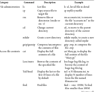
TABLE 1.1 Common Basic Linux Commands
Category Command Description Example
File administration ls List files ls -al, list all file in detail cp Copy source file to
target file
cp myfile yourfile
rm Remove files or directories (rmdir or rm -r)
rm accounts.txt, to remove the file “accounts.txt” in the current directory
cd Change current directory
cd., to move to the parent directory of the current directory
mkdir Create a new directory mkdir mydir, to create a new directory called mydir gzip/gunzip Compress/uncompress
the contents of files
gzip .swp, to compress the file .swp
Access file contents cat Display the full contents of a file
cat Mary.py, to display the full content of the file “Mary.py”
Less/more Browse the contents of the specified file
less huge-log-file.log, to browse the content of huge-log-file.log Tail/head Display the last or the
first 10 lines of a file by default
tail -n N filename.txt, to display N number of lines from the file named filename.txt
find Find files find ~ -size -100M, To find files smaller than 100M
8 ◾ Big Data Analysis for Bioinformatics and Biomedical Discoveries
followed by the name of the command, for example, man ls, which will show how to list files in various ways.
1.2.3 File Access Permission
On Linux and other Unix-like operating systems, there is a set of rules for each file, which defines who can access that file and how they can access it. These rules are called file permissions or file modes. The command name chmod stands for change mode, and it is used to define the way a file can be accessed. For example, if one issues a command line to a file named Mary.py like chmod 765 Mary.py, the permission is indicated by -rwxrw-r-x, which allows the user to read (r), write (w), and execute (x), the group to read and write, and any other to read and execute the file. The chmod numerical format (octal modes) is presented in Table 1.2.
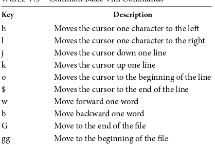
1.2.4 Linux Text Editors
Text editors are needed to write scripts. There are a number of available text editors such as Emacs, Eclipse, gEdit, Nano, Pico, and Vim. Here we briefly introduce Vim, a very popular Linux text editor. Vim is the editor of choice for many developers and power users. It is based on the vi editor written by Bill Joy in the 1970s for a version of UNIX. It inherits the key bindings of vi, but also adds a great deal of functionality and extensibility that are missing from the original vi. You can start Vim editor by typing vim followed with a file name. After you finish the text file, you can type
TABLE 1.1 (CONTINUED) Common Basic Linux Commands
Category Command Description Example
grep Search for a specific string in the specified file
grep “this” demo_file, to search “this” containing sentences from the “demo_file” Processes top Provide an ongoing
look at processor activity in real time
top –s, to work in secure mode
kill Shut down a process kill -9, to send a KILL signal instead of a TERM signal System information df Display disk space df –H, to show the number
of occupied blocks in human-readable format free Display information
about RAM and swap space usage
Linux for Big Data Analysis ◾ 9
semicolon (:) plus a lower case letter x to save the file and exit Vim editor. Table 1.3 lists the most common basic commands used in the Vim editor.
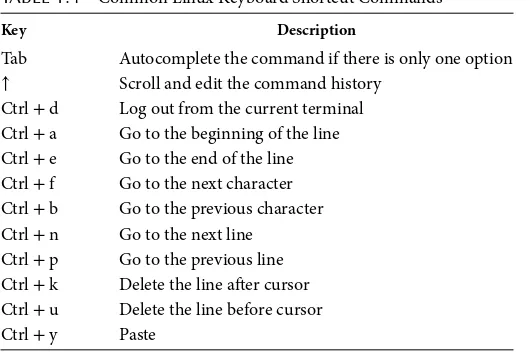
1.2.5 Keyboard Shortcuts
The command line can be quite powerful, but typing in long commands or file paths is a tedious process. Here are some shortcuts that will have you running long, tedious, or complex commands with just a few key-strokes (Table 1.4). If you plan to spend a lot of time at the command line, these shortcuts will save you a ton of time by mastering them. One should become a computer ninja with these time-saving shortcuts.
1.2.6 Write Shell Scripts
A shell script is a computer program or series of commands written in plain text file designed to be run by the Linux/Unix shell, a command-line interpreter. Shell scripts can automate the execution of repeated tasks and save lots of time. Shell scripts are considered to be scripting languages
TABLE 1.3 Common Basic Vim Commands
Key Description
h Moves the cursor one character to the left l Moves the cursor one character to the right j Moves the cursor down one line
k Moves the cursor up one line
o Moves the cursor to the beginning of the line $ Moves the cursor to the end of the line w Move forward one word
b Move backward one word G Move to the end of the file gg Move to the beginning of the file
TABLE 1.2 The chmod Numerical Format (Octal Modes)
Number Permission rwx
7 Read, write, and execute 111 6 Read and write 110 5 Read and execute 101
4 Read only 100
3 Write and execute 011
2 Write only 010
1 Execute only 001
10 ◾ Big Data Analysis for Bioinformatics and Biomedical Discoveries
or programming languages. The many advantages of writing shell scripts include easy program or file selection, quick start, and interactive debug-ging. Above all, the biggest advantage of writing a shell script is that the commands and syntax are exactly the same as those directly entered at the command line. The programmer does not have to switch to a totally differ-ent syntax, as they would if the script was written in a differdiffer-ent language or if a compiled language was used. Typical operations performed by shell scripts include file manipulation, program execution, and printing text. Generally, three steps are required to write a shell script: (1) Use any edi-tor like Vim or others to write a shell script. Type vim first in the shell prompt to give a file name first before entering the vim. Type your first script as shown in Figure 1.2a, save the file, and exit Vim. (2) Set execute
TABLE 1.4 Common Linux Keyboard Shortcut Commands
Key Description
Tab Autocomplete the command if there is only one option
↑ Scroll and edit the command history Ctrl + d Log out from the current terminal Ctrl + a Go to the beginning of the line Ctrl + e Go to the end of the line Ctrl + f Go to the next character Ctrl + b Go to the previous character Ctrl + n Go to the next line
Ctrl + p Go to the previous line Ctrl + k Delete the line after cursor Ctrl + u Delete the line before cursor Ctrl + y Paste
(a) #
# My first shell script #
clear
echo “Next generation DNA sequencing increases the speed and reduces the cost of DNA sequencing relative to the first generation DNA sequencing.”
(b)
Next generation DNA sequencing increases the speed and reduces the cost of DNA sequencing relative to the first generation DNA sequencing
Linux for Big Data Analysis ◾ 11
permission for the script as follows: chmod 765 first, which allows the user to read (r), write (w), and execute (x), the group to read and write, and any other to read and execute the file. (3) Execute the script by typing: ./first. The full script will appear as shown in Figure 1.2b.
1.3 STEP-BY-STEP TUTORIAL ON NEXT- GENERATION
SEQUENCE DATA ANALYSIS BY RUNNING
BASIC LINUX COMMANDS
By running Linux commands, this tutorial demonstrates a step-by-step general procedure for next-generation sequence data analysis by first retrieving or downloading a raw sequence file from NCBI/NIH Gene Expression Omnibus (GEO, http://www.ncbi.nlm.nih.gov/geo/); second, exercising quality control of sequences; third, mapping sequencing reads to a reference genome; and fourth, visualizing data in a genome browser. This tutorial assumes that a user of a desktop or laptop computer has an Internet connection and an SSH such as PuTTY, which can be logged onto a Linux-based high-performance computer cluster with needed software or programs. All the following involved commands in this tutorial are supposed to be available in your current directory, like /home/username. It should be mentioned that this tutorial only gives you a feel on next-gen-eration sequence data analysis by running basic Linux commands and it won’t cover complete pipelines for next-generation sequence data analysis, which will be detailed in subsequent chapters.
1.3.1 Step 1: Retrieving a Sequencing File
12 ◾ Big Data Analysis for Bioinformatics and Biomedical Discoveries
1.3.1.1 Locate the File
Go to the GEO site (http://www.ncbi.nlm.nih.gov/geo/) → select Search GEO Datasets from the dropdown menu of Query and Browse → type GSE45732 in the Search window → click the hyperlink (Gene expression analysis of breast cancer cell lines) of the first choice → scroll down to the bottom to locate the SRA file (SRP/SRP020/SRP020493) prepared for ftp download → click the hyperlynx(ftp) to pinpoint down the detailed ftp address of the source file (SRR805877, ftp://ftp-trace.ncbi.nlm.nih. gov/sra/sra-instant/reads/ByStudy/sra/SRP%2FSRP020%2FSRP020493/ SRR805877/).
1.3.1.2 Downloading the Short-Read Sequencing File (SRR805877) from NIH GEO Site
Type the following command line in the shell prompt: “wget ftp://ftp-trace. ncbi.nlm.nih.gov/sra/sra-instant/reads/ByStudy/sra/SRP%2FSRP020% 2FSRP020493 /SRR805877/SRR805877.sra.”
1.3.1.3 Using the SRA Toolkit to Convert .sra Files into .fastq Files
FASTQ formatis a text-based format for storing both a biological sequence (usually nucleotide sequence) and its corresponding quality scores. It has become the de facto standard for storing the output of high-throughput sequencing instruments such as the Illumina’s HiSeq 2500 sequencing system. Type “fastq-dump SRR805877.sra” in the command line. SRR805877.fastq will be produced. If you download paired-end sequence data, the parameter “-I” appends read id after spot id as “accession.spot.readid” on defline and the parameter “--split-files” dump each read into a separate file. Files will receive a suffix corresponding to its read number. It will produce two fastq files (--split-files) containing “.1” and “.2” read suffices (-I) for paired-end data.
1.3.2 Step 2: Quality Control of Sequences
Before doing analysis, it is important to ensure that the data are of high quality. FASTQC can import data from FASTQ, BAM, and Sequence Alignment/Map (SAM) format, and it will produce a quick overview to tell you in which areas there may be problems, summary graphs, and tables to assess your data.
1.3.2.1 Make a New Directory “Fastqc”
Linux for Big Data Analysis ◾ 13
1.3.2.2 Run “Fastqc”
Type “fastqc -o Fastqc/SRR805877.fastq” in the command line, which will run Fastqc to assess SRR805877.fastq quality. Type “Is -l Fastqc/,” you will see the results in detail.
1.3.3 Step 3: Mapping Reads to a Reference Genome
At first, you need to prepare genome index and annotation files. Illumina has provided a set of freely downloadable packages that contain bow-tie indexes and annotation files in a general transfer format (GTF) from UCSC Genome Browser Home (genome.ucsc.edu).
1.3.3.1 Downloading the Human Genome and Annotation from Illumina iGenomes
Type “wget ftp://igenome:[email protected]/Homo_ sapiens/UCSC/hg19/Homo_sapiens_UCSC_hg19.tar.gz” and download those files.
1.3.3.2 Decompressing .tar.gz Files
Type “tar -zxvf Homo_sapiens_Ensembl_GRCh37.tar.gz” for extracting the files from archive.tar.gz.
1.3.3.3 Link Human Annotation and Bowtie Index to the Current Working Directory
Type “In -s homo.sapiens/UCSC/hg19/Sequence/WholeGenomeFasta/ genome.fa genome.fa”; type “In -s homo.sapiens/UCSC/hg19/Sequence/ Bowtie2Index/genome.1.bt2 genome.1.bt2”; type “In -s homo.sapiens/ UCSC/hg19/Sequence/Bowtie2Index/genome.2.bt2 genome.2.bt2”; type “In -s homo.sapiens/UCSC/hg19/Sequence/Bowtie2Index/genome.3.bt2 genome.3.bt2”; type “In -s homo.sapiens/UCSC/hg19/Sequence/Bowtie2 Index/genome.4.bt2 genome.4.bt2”; type “In -s homo.sapiens/UCSC/hg19/ Sequence/Bowtie2Index/genome.rev.1.bt2 genome.rev.1.bt2”; type “In -s homo.sapiens/UCSC/hg19/Sequence/Bowtie2Index/genome.rev.2.bt2 genome.rev.2.bt2”; and type “In -s homo.sapiens/UCSC/hg19/Annotation/ Genes/genes.gtf genes.gtf.”
1.3.3.4 Mapping Reads into Reference Genome
14 ◾ Big Data Analysis for Bioinformatics and Biomedical Discoveries
1.3.4 Step 4: Visualizing Data in a Genome Browser
The primary output of TopHat are the aligned reads BAM file and junc-tions BED file, which allows read alignments to be visualized in genome browser. A BAM file (*.bam) is the compressed binary version of a SAM file that is used to represent aligned sequences. BED stands for Browser Extensible Data. A BED file format provides a flexible way to define the data lines that can be displayed in an annotation track of the UCSC Genome Browser. You can choose to build a density graph of your reads across the genome by typing the command line: “genomeCoverageBed -ibam tophat/accepted_hits.bam -bg -trackline -trackopts ‘name=“SRR805877” color=250,0,0’>SRR805877.bedGraph” and run. For convenience, you need to transfer these output files to your desktop computer’s hard drive.
1.3.4.1 Go to Human (Homo sapiens) Genome Browser Gateway
You can load bed or bedGraph into the UCSC Genome Browser to visu-alize your own data. Open the link in your browser: http://genome.ucsc. edu/cgi-bin/hgGateway?hgsid=409110585_zAC8Aks9YLbq7YGhQiQtw nOhoRfX&clade=mammal&org=Human&db=hg19.
1.3.4.2 Visualize the File
Click on add custom tracks button → click on Choose File button, and select your file → click on Submit button → click on go to genome browser. BED files will provide the coordinates of regions in a genome; most basi-cally chr, start, and end. bedGraph files can give coordinate information as in BED files and coverage depth of sequencing over a genome.
BIBLIOGRAPHY
1. Haas, J. Linux, the Ultimate Unix, 2004, http://linux.about.com/cs/linux101/ a/linux_2.htm.
2. Gite, VG. Linux Shell Scripting Tutorial v1.05r3-A Beginner’s Handbook, 1999–2002, http://www.freeos.com/guides/lsst/.
3. Brockmeier, J.Z. Vim 101: A Beginner’s Guide to Vim, 2009, http://www. linux.com/learn/tutorials/228600-vim-101-a-beginners-guide-to-vim. 4. Chris Benner et al. HOMER (v4.7), Software for motif discovery and next
generation sequencing analysis, August 25, 2014, http://homer.salk.edu/ homer/basicTutorial/.
5. Shotts, WE, Jr. The Linux Command Line: A Complete Introduction, 1st ed., No Starch Press, January 14, 2012.
15 C H A P T E R
2
Python for Big
Data Analysis
Dmitry N. Grigoryev
2.1 INTRODUCTION TO PYTHON
Python is a powerful, flexible, open-source programming language that is easy to use and easy to learn. With the help of Python you will be able to manipulate large data sets, which is hard to do with common data oper-ating programs such as Excel. But saying this, you do not have to give up your friendly Excel and its familiar environment! After your Big Data manipulation with Python is completed, you can convert results back to your favorite Excel format. Of course, with the development of technology at some point, Excel would accommodate huge data files with all known genetic variants, but the functionality and speed of data processing by Python would be hard to match. Therefore, the basic knowledge of pro-gramming in Python is a good investment of your time and effort. Once you familiarize yourself with Python, you will not be confused with it or intimidated by numerous applications and tools developed for Big Data analysis using Python programming language.
CONTENTS
2.1 Introduction to Python 15
2.2 Application of Python 16
2.3 Evolution of Python 16
2.4 Step-By-Step Tutorial of Python Scripting in UNIX
and Windows Environments 17
2.4.1 Analysis of FASTQ Files 17
2.4.2 Analysis of VCF Files 21
16 ◾ Big Data Analysis for Bioinformatics and Biomedical Discoveries
2.2 APPLICATION OF PYTHON
There is no secret that the most powerful Big Data analyzing tools are written in compiled languages like C or java, simply because they run faster and are more efficient in managing memory resources, which is cru-cial for Big Data analysis. Python is usually used as an auxiliary language and serves as a pipeline glue. The TopHat tool is a good example of it [1]. TopHat consists of several smaller programs written in C, where Python is employed to interpret the user-imported parameters and run small C programs in sequence. In the tutorial section, we will demonstrate how to glue together a pipeline for an analysis of a FASTQ file.
However, with fast technological advances and constant increases in computer power and memory capacity, the advantages of C and java have become less and less obvious. Python-based tools have started taking over because of their code simplicity. These tools, which are solely based on Python, have become more and more popular among researchers. Several representative programs are listed in Table 2.1.
As you can see, these tools and programs cover multiple areas of Big Data analysis, and number of similar tools keep growing.
2.3 EVOLUTION OF PYTHON
Python’s role in bioinformatics and Big Data analysis continues to grow. The constant attempts to further advance the first-developed and most popular set of Python tools for biological data manipulation, Biopython (Table 2.1), speak volumes. Currently, Biopython has eight actively devel-oping projects (http://biopython.org/wiki/Active_projects), several of which will have potential impact in the field of Big Data analysis.
TABLE 2.1 Python-Based Tools Reported in Biomedical Literature
Tool Description Reference
Biopython Set of freely available tools for biological computation
Cock et al. [2]
Galaxy An open, web-based platform for data intensive biomedical research
Goecks et al. [3]
msatcommander Locates microsatellite (SSR, VNTR, &c) repeats within FASTA-formatted sequence or consensus files
Faircloth et al. [4]
RseQC Comprehensively evaluates high-throughput sequence data especially RNA-seq data
Wang et al. [5]
Chimerascan Detects chimeric transcripts in high-throughput sequencing data
Python for Big Data Analysis ◾ 17
The perfect example of such tool is a development of a generic feature format (GFF) parser. GFF files represent numerous descriptive features and annotations for sequences and are available from many sequenc-ing and annotation centers. These files are in a TAB delimited format, which makes them compatible with Excel worksheet and, therefore, more friendly for biologists. Once developed, the GFF parser will allow analysis of GFF files by automated processes.
Another example is an expansion of Biopython’s population genetics (PopGen) module. The current PopGen tool contains a set of applications and algorithms to handle population genetics data. The new extension of PopGen will support all classic statistical approaches in analyzing popula-tion genetics. It will also provide extensible, easy-to-use, and future-proof framework, which will lay ground for further enrichment with newly developed statistical approaches.
As we can see, Python is a living creature, which is gaining popularity and establishing itself in the field of Big Data analysis. To keep abreast with the Big Data analysis, researches should familiarize themselves with the Python programming language, at least at the basic level. The follow-ing section will help the reader to do exactly this.
2.4 STEP-BY-STEP TUTORIAL OF PYTHON SCRIPTING
IN UNIX AND WINDOWS ENVIRONMENTS
Our tutorial will be based on the real data (FASTQ file) obtained with Ion Torrent sequencing (www.lifetechnologies.com). In the first part of the tutorial, we will be using the UNIX environment (some tools for pro-cessing FASTQ files are not available in Windows). The second part of the tutorial can be executed in both environments. In this part, we will revisit the pipeline approach described in the first part, which will be demon-strated in the Windows environment. The examples of Python utility in this tutorial will be simple and well explained for a researcher with bio-medical background.
2.4.1 Analysis of FASTQ Files
18 ◾ Big Data Analysis for Bioinformatics and Biomedical Discoveries
and also ask to have the reference genome and tools listed in Table 2.2 installed. Once we have everything in place, we can begin our tutorial with the introduction to the pipelining ability of Python. To answer the potential question of why we need pipelining, let us consider the fol-lowing list of required commands that have to be executed to analyze a FASTQ file. We will use a recent publication, which provides a resource of benchmark SNP data sets [7] and a downloadable file bb17523_PSP4_ BC20.fastq from ftp://ftp-trace.ncbi.nih.gov/giab/ftp/data/NA12878/ion_ exome. To use this file in our tutorial, we will rename it to test.fastq.
In the meantime, you can download the human hg19 genome from Illumina iGenomes (ftp://igenome:G3nom3s4u@ussd-ftp.illumina.com/ Homo_sapiens/UCSC/hg19/Homo_sapiens_UCSC_hg19.tar.gz). The files are zipped, so you need to unpack them.
In Table 2.2, we outline how this FASTQ file should be processed. Performing the steps presented in Table 2.2 one after the other is a labo-rious and time-consuming task. Each of the tools involved will take some-where from 1 to 3 h of computing time, depending on the power of your computer. It goes without saying that you have to check on the progress of your data analysis from time to time, to be able to start the next step. And, of course, the overnight time of possible computing will be lost, unless somebody is monitoring the process all night long. The pipelining with Python will avoid all these trouble. Once you start your pipeline, you can forget about your data until the analysis is done, and now we will show you how.
For scripting in Python, we can use any text editor. Microsoft (MS) Word will fit well to our task, especially given that we can trace the whitespaces of
TABLE 2.2 Common Steps for SNP Analysis of Next-Generation Sequencing Data
Step Tool Goal Reference
1 Trimmomatic To trim nucleotides with bad quality from the ends of a FASTQ file
Bolger et al. [8]
2 PRINSEQ To evaluate our trimmed file and select reads with good quality
Schmieder et al. [9]
3 BWA-MEM To map our good quality sequences to a reference genome
Li et al. [10]
4
SAMtools To generate a BAM file and sort it Li et al. [11] 5 To generate a MPILEUP file
Python for Big Data Analysis ◾ 19
our script by making them visible using the formatting tool of MS Word. Open a new MS Word document and start programming in Python! To create a pipeline for analysis of the FASTQ file, we will use the Python col-lection of functions named subprocess and will import from this colcol-lection function call.
The first line of our code will be
from subprocess import call
Now we will write our first pipeline command. We create a variable, which you can name at will. We will call it step_1 and assign to it the desired pipeline command (the pipeline command should be put in quotation marks and parenthesis):
step_1 = (“java -jar ~/programs/Trimmomatic-0.32/ trimmomatic-0.32.jar SE -phred33 test.fastq test_trmd. fastq LEADING:25 TRAILING:25 MINLEN:36”)
Note that a single = sign in programming languages is used for an assign-ment stateassign-ment and not as an equal sign. Also note that whitespaces are very important in UNIX syntax; therefore, do not leave any spaces in your file names. Name your files without spaces or replace spaces with underscores, as in test_trimmed.fastq. And finally, our Trimmomatic tool is located in the programs folder, yours might have a different location. Consult your administrator, where all your tools are located.
Once our first step is assigned, we would like Python to display variable step_1 to us. Given that we have multiple steps in our pipeline, we would like to know what particular step our pipeline is running at a given time. To trace the data flow, we will use print() function, which will display on the monitor what step we are about to execute, and then we will use call() function to execute this step:
print(step_1)
call(step_1, shell = True)
20 ◾ Big Data Analysis for Bioinformatics and Biomedical Discoveries
from subprocess import call
step_1 = (“java -jar ~/programs/Trimmomatic-0.32/ trimmomatic-0.32.jar SE -phred33 test.fastq test_ trimmed.fastq LEADING:25 TRAILING:25 MINLEN:36”) print(step_1)
call(step_1, shell = True)
step_2 = (“perl ~/programs/prinseq-lite-0.20.4/ prinseq-lite.pl -fastq test_trimmed.fastq -min_qual_ mean 20 -out_good test_good”)
print(step_2)
call(step_2, shell = True)
step_3 = (“bwa mem -t 20 homo.sapiens/UCSC/hg19/ Sequence/BWAIndex/genome.fa test_good.fastq > test_ good.sam”)
print(step_3)
call(step_3, shell = True)
step_4 = (“samtools view –bS test_good.sam > test_ good.bam”)
print(step_4)
call(step_4, shell = True)
step_5 = (“samtools sort test_good.bam test_good_sorted”)
print(step_5)
call(step_5, shell = True)
step_6 = (“samtools mpileup –f homo.sapiens/UCSC/ hg19/Sequence/WholeGenomeFasta/genome.fa test_good_ sorted.bam > test_good.mpileup”)
print(step_6)
call(step_6, shell = True)
step_7 = (“java -jar ~/programs/VarScan.v2.3.6.jar mpileup2snp test_good.mpileup --output-vcf 1 >
test. vcf”) print(step_7)
call(step_7, shell = True)
Now we are ready to go from MS Word to a Python file. In UNIX, we will use vi text editor and name our Python file pipeline.py, where extension .py will tell that this is a Python file.
In UNIX command line type: vi pipeline.py
Python for Big Data Analysis ◾ 21
button and select from the popup menu Paste. While inside the vi text editor, turn off the INSERT mode by pressing the Esc key. Then type ZZ, which will save and close pipeline.py file. The quick tutorial for the vi text editor can be found at http://www.tutorialspoint.com/unix/unix-vi-editor.htm.
Once our pipeline.py file is created, we will run it with the command:
python pipeline.py
This script is universal and should processs any FASTQ file.
2.4.2 Analysis of VCF Files
To be on the same page with those who do not have access to UNIX and were not able to generate their own VCF file, we will download the premade VCF file TSVC_variants.vcf from the same source (ftp://ftp-trace.ncbi.nih. gov/giab/ftp/data/NA12878/ion_exome), and will rename it to test.vcf.
From now on we will operate on this test.vcf file, which can be analyzed in both UNIX and Windows environments. You can look at this test.vcf files using the familiar Excel worksheet. Any Excel version should accom-modate our test.vcf file; however, if you try to open a bigger file, you might encounter a problem. Excel will tell that it cannot open the whole file. If you wonder why, the answer is simple. If, for example, you are working with MS Excel 2013, the limit of rows for a worksheet in this version will be 1,048,576. It sounds like a lot, but wait, to accommodate all SNPs from the whole human genome the average size of a VCF file will need to be up to 1,400,000 rows [13]. Now you realize that you have to manipulate your file by means other than Excel. This is where Python becomes handy. With its help you can reduce the file size to manageable row numbers and at the same time retain meaningful information by excluding rows without variant calls.
22 ◾ Big Data Analysis for Bioinformatics and Biomedical Discoveries
fantasy desires. We will keep it simple and name it file. Now we will use function open() to open our file. To make sure that this file will not be accidently altered in any way, we will use argument of open() function ‘r’, which allows Python only to read this file. At the same time, we will cre-ate an output file and call it newfile. Again, we will use function open() to create our new file with name test_no_description_1.vcf. To tell Python that it can write to this file, we will use argument of open() function ‘w’:
file = open(“test.vcf”,‘r’)
newfile = open(“test_no_description_1.vcf”,‘w’)
Now we will create all variables that are required for our task. In this script, we will need only two of them. One we will call line and the other—
n, where line will contain information about components of each row in test.vcf, and n will contain information about the sequential number of a row. Given that line is a string variable (contains string of characters), we will assign to it any string of characters of your choosing. Here we will use “abc.” This kind of variable is called character variable and its content should be put in quotation marks. The n variable on the other hand will be a numeric variable (contains numbers); therefore, we will assign a number to it. We will use it for counting rows, and given that we do not count any rows yet, we assign 0 to n without any quotation marks.
line = “abc” n = 0
Now we are ready for the body of the script. Before we start, we have to outline the whole idea of the script function. In our case, the script should read the test.vcf file line by line and write all but the first 64 lines to a new file. To read the file line by line, we need to build a repetitive structure—in programming world this is called loops. There are several loop structures in Python, for our purpose we will use the “while” structure. A Python while loop behaves quite similarly to common English. Presumably, you would count the pages of your grant application. If a page is filled with the text from top to bottom, you would count this page and go to the next page. As long as your new page is filled up with the text, you would repeat your action of turning pages until you reach the empty page. Python has a similar syntax: while line != “”:
Python for Big Data Analysis ◾ 23
block of code (body of the loop). Note that each statement in Python (in our case looping statement) should be completed with the colon sign (:). Actually, this is the only delimiter that Python has. Python does not use delimiters such as curly braces to mark where the function code starts and stops as in other programming languages. What Python uses instead is indentations. Blocks of code in Python are defined by their indenta-tion. By block of code, in our case we mean the content of the body of our “while” loop. Indenting the starts of a block and unindenting ends it. This means that whitespaces in Python are significant and must be consistent. In our example, the code of loop body will be indented six spaces. It does not need to be exactly six spaces, it has to be at least one, but once you have selected your indentation size, it needs to be consistent. Now we are going to populate out while loop. As we have decided above, we have to read the content of the first row from test.vcf. For this we will use function read-line(). This function should be attached to a file to be read via a point sign. Once evoked, this function reads the first line of provided file into variable line and automatically jumps to the next line in the file.
line = file.readline() n = n + 1
To keep track of numbers for variable line, we started up our counter n. Remember, we set n to 0. Now our n is assigned number 1, which corre-sponds to our row number. With each looping, n will be increasing by 1 until the loop reaches the empty line, which is located right after the last populated line of test.vcf.
Now we have to use another Python structure: if-else statement.
if n <= 64: continue else:
newfile.write(line)
24 ◾ Big Data Analysis for Bioinformatics and Biomedical Discoveries
the colon (:). The block of if statement (in our case continue) is indented, which means that it will be executed only when the condition in the if statement is true. Once we went over the line number 64, we want the rest of the test.vcf file to be written to our new file. Here we used the write() function. As with readline() function, we attached write() func-tion to a file to be written to via a point sign. Inside of the parenthesis of a function, we put the argument line to let the function know what to write to the newfile. Note that the logical else statement is also com-pleted with the colon (:). The block of else statement (newfile.write(line) in our case) is indented, which means that it will be executed only when the original condition, if n <= 64, is false. In an if-else statement, only one of two indented blocks can be executed. Once we run our loop and generated a file, which does not have 64 descriptive rows in it, we can close both original and newly generated files. To do this, we will use function close(). Once again, we will attach close() function to a file to be closed via a point sign.
newfile.close() file.close()
Python for Big Data Analysis ◾ 25
Make sure that your step_1a.py file and test.vcf file are located in the same directory. Once we have familiarized ourselves with Python script-ing, we will move to a more complex task. As we said above, there are two ways to code for removing descriptive rows from a VCF file. One can ask: why do we need another approach to perform this file modification? The answer is: not all VCF files are created in the same way. Although, by convention, all descriptive rows in VCF files begin with double pound sign (##), the number of descriptive rows varies from one sequence align-ing program to another. For instance, VСF files generated by Genome Analysis Toolkit for FASTQ files from Illumina platform have 53 tive rows [13] and our pipeline described above will generate 23 descrip-tive rows. Of course, we can change our logical statement if n <= 64: to if n <= 53: or if n <= 23:, but why do not make our code universal? We already know that each descriptive row in VCF files begin with ## sign; therefore, we can identify and remove them. Given that we are planning to manipulate on the row content, we have to modify our loop. Our previ-ous script was taking the empty row at the end of the test.vcf file and was writing it to the test_no_description_1.vcf file without looking into the row content. Now, when we operate on the content of a row, Python will complain about the empty content and will report an error. To avoid this, we have to make sure that our script does not operate with the empty row. To do this, we will check whether the row is empty beforehand, and if it is, we will use break statement to abort our script. Once again, our code will
26 ◾ Big Data Analysis for Bioinformatics and Biomedical Discoveries
be close to English. Assume you are proofreading your completed grant application. If you reach the end of it and see the empty page, you are done and deserve a break.
if line == “”: break
As you might have noticed, we used just part of the if-else statement, which is perfectly legal in Python. Once our program reaches the end of the file, there is nothing else to do but stop the script with break statement; there-fore, there is no need for any else. And another new sign double equal (==) stands for a regular equal. Note that even the shortened if-else statement should be completed with the colon (:). The block of the if statement (in our case break) also should be indented, which means that it will be executed only when the condition in the if statement is true. Now, when we created internal break, we do not need the redundant check point at the beginning of our loop. Therefore, we will replace while line != “”: with while 1:. Here we have introduced the “infinite” loop. The statement while 1 will run our loop forever unless we stop it with a break statement. Next, we will modify our existing if-else statement. Given that now we are searching for a ## pattern inside the row, rather than simply counting rows, we will replace
if n <= 64: with
if line[1] == “#”:
With line[1], we introduce the process of counting row content in Python. The line variable here represents the whole row of test.vcf file. To visual-ize content of a line variable, you can simply display it on your computer screen with print() function using line as an argument.
file = open(“test.vcf”,‘r’) line = file.readline() print(line)
Python for Big Data Analysis ◾ 27
number into square brackets, for example, command print(line[1]) will display the second # sign. This is our mark for the descriptive rows; there-fore, whenever our script sees line[1] as #, it will skip this row and go to the next one. Our complete modified script will look like this now:
print(“START”)
file = open(“test.vcf”,‘r’)
newfile = open(“test_no_description_2.vcf”,‘w’) line = “abc”
while 1:
line = file.readline()
if line == “”: break
if line[1] == “#”: continue else:
newfile.write(line) newfile.close()
file.close() print(“END”)
Now we can copy and paste our script either into vi text editor (UNIX) or into Python GUI Shell (Windows), save it as step_1b.py and run. Once we are done with cutting out the descriptive rows, we can further simplify and reduce the size of our VCF file. We will use our previous script as template, and for the beginning, we will change our input and output files. Given that our goal is to make original VCF file the Excel compatible, we will use text format for our output file and will add to the file name an extension .txt.
file = open(“test_no_description_2.vcf”,‘r’) newfile = open(“alleles.txt”,‘w’)
28 ◾ Big Data Analysis for Bioinformatics and Biomedical Discoveries
# Creating columns titles for newfile
line = file.readline()
newfile.write(“Chromosome” + “\t” + “Position” + “\t” +
“Alleles” + “\n”)
Given that columns in text formatted files are separated by the TAB sign (\t), we separated our titles with “\t,” and, as we learned by now, all textual entries in Python should have quotation marks. We also have to end the title row with the NEWLINE sign (\n), which tells Python that this row is completed and any further input should go to the next row. Once we are done with formatting our output file, we will restructure our existing if-else statement by adding new variable. This variable (we will call it rec) will keep record of each column content after we split a row by columns. To manipulate the row content on column-by-column bases, we will need a package of functions specifically designed to do exactly this. The package is called string. In our first pipeline exercise, we already had an experience with importing call function; here in the same fashion, we will import string using an identical Python statement: import string.
Now we are set to operate on the row content. Before we begin, we have to check how many columns the file we are going to operate on has. By convention, a VCF file has nine mandatory columns, and then starting with the tenth column, it will have one sample per column. For simplicity, in our tutorial, we have a VCF file with just one sample. We also have to know what kind of column separator is used in our data. By convention, a VCF file uses tab (\t) as a column separator. Armed with this knowledge, we can start scripting. First, we read the whole row from our file, assign it to the variable line, and will make sure that this line is not empty. Then, we will split the line in pieces according to columns using the string splitting function str.split():
line = file.readline() if line == “”:
break
rec = str.split(line,“\t”)
Python for Big Data Analysis ◾ 29
counting starts with 0. Therefore, the tenth column in our row for Python will be column number nine. To display the content of the column 10, where our sample sits, we will use print() function: print(rec[9]).
In our exercise, you will see on your computer screen the following row of data:
1/1:87:92:91:0:0:91:91:43:48:0:0:43:48:0:0
Before going further, we have to familiarize ourselves with the format of VCF file. For the detailed explanation of its format, the reader can use Genome 1000 website (http://samtools.github.io/hts-specs/VCFv4.2.pdf). For our purpose, we will consider only the genotype part of the VCF file, which is exactly what we are seeing on our screens right now.
Genotype of a sample is encoded as allele values separated by slash (/). The allele values are 0 for a reference allele (which is provided in the REF column—column four or rec[3]) and 1 for the altered allele (which is provided in the ALT column—column five or rec[4]). For homozygote calls, examples could be either 0/0 or 1/1, and for heterozygotes either 0/1 or 1/0. If a call cannot be made for a sample at a given locus, each missing allele will be specified with a point sign (./.). With this knowl-edge in hands, the reader can deduce that in order to identify genotype of a sample we are going to operate on the first and the third elements of rec[9] (row of data above), which are representing codes for alleles iden-tified by sequencing (in our example 1 and 1 or ALT and ALT alleles, respectively). But once again for Python these are not positions 1 and 3, but rather 0 and 2; therefore, we tell Python that we would like to work on rec[9][0] and rec[9][2]. Now we are set with the values to work with and can resume scripting. First, we will get rid of all meaningless allele calls, which are coded with points instead of numbers (./.). Using the similar construction, which we used above for skipping descriptive rows, we will get this statement:
if rec[9][0] == “.” or rec[9][2] == “.”: continue
30 ◾ Big Data Analysis for Bioinformatics and Biomedical Discoveries
The script will return to the beginning of while loop and will start analysis of the next row in test_no_description_2.vcf file. Now we have to con-sider a situation when both alleles were identified by a sequencer and were assigned corresponding code, either 0 or 1. In this case, the script should write a new row to our output file. Therefore, we have to start to build this row beginning with the variant location in the genome. In our input file, this information is kept in the first two columns “Chromosome” and “Position,” which are for Python rec[0] and rec[1].
newfile.write(rec[0] + “\t” + rec[1] + “\t”)
Here we follow the same rule as for a title row and separating future columns by TAB (\t) character. Now we have to populate the third column of our output file with allelic information. Analyzing structure of our VCF file, we already figured out that reference allele is corresponding to rec[3] and altered allele is corresponding to rec[4]. Therefore, our script for writ-ing first allele will be
# Working with the first allele if rec[9][0] == “0”:
newfile.write(rec[3]) else:
newfile.write(rec[4])
We comment to ourselves that we are working with the first allele (rec[9] [0]). These lines of script tell that if an allele is coded by 0, it will be presented in the “Alleles” column as the reference allele (rec[3]), otherwise (else) it will be presented as the altered allele (rec[4]). And how do we know that we have only two choices? Because we have already got rid of non-called alleles (./.) and the rec[9][0] can only be 0 or 1. The second allele (rec[9][2]) will be processed in the same fashion (the only difference will be an addition of the NEWLINE character /n), and our complete script will be as follows:
print(“START”) import string
file = open(“test_no_description_2.vcf”,‘r’) newfile = open(“alleles.txt”,‘w’)
line = “abc”