Data Science Fundamentals for Python and MongoDB pdf pdf

(1)

Data Science

Fundamentals

for Python and

MongoDB

(2)

Data Science

Fundamentals for

Python and MongoDB

(3)

ISBN-13 (pbk): 978-1-4842-3596-6 ISBN-13 (electronic): 978-1-4842-3597-3 https://doi.org/10.1007/978-1-4842-3597-3

This work is subject to copyright. All rights are reserved by the Publisher, whether the whole or part of the material is concerned, specifically the rights of translation, reprinting, reuse of illustrations, recitation, broadcasting, reproduction on microfilms or in any other physical way, and transmission or information storage and retrieval, electronic adaptation, computer software, or by similar or dissimilar methodology now known or hereafter developed. Trademarked names, logos, and images may appear in this book. Rather than use a trademark symbol with every occurrence of a trademarked name, logo, or image, we use the names, logos, and images only in an editorial fashion and to the benefit of the trademark owner, with no intention of infringement of the trademark.

The use in this publication of trade names, trademarks, service marks, and similar terms, even if they are not identified as such, is not to be taken as an expression of opinion as to whether or not they are subject to proprietary rights.

While the advice and information in this book are believed to be true and accurate at the date of publication, neither the authors nor the editors nor the publisher can accept any legal responsibility for any errors or omissions that may be made. The publisher makes no warranty, express or implied, with respect to the material contained herein.

Managing Director, Apress Media LLC: Welmoed Spahr Acquisitions Editor: Jonathan Gennick

Development Editor: Laura Berendson Coordinating Editor: Jill Balzano Cover designed by eStudioCalamar

Cover image designed by Freepik (www.freepik.com)

Distributed to the book trade worldwide by Springer Science+Business Media New York, 233 Spring Street, 6th Floor, New York, NY 10013. Phone 1-800-SPRINGER, fax (201) 348-4505, e-mail orders-ny@springer-sbm.com, or visit www.springeronline.com. Apress Media, LLC is a California LLC and the sole member (owner) is Springer Science + Business Media Finance Inc (SSBM Finance Inc). SSBM Finance Inc is a Delaware corporation. For information on translations, please e-mail rights@apress.com, or visit

http://www.apress.com/rights-permissions.

Apress titles may be purchased in bulk for academic, corporate, or promotional use. eBook David Paper

(4)

Moonbeam whose support and love is and always has been

unconditional. To the Apress staff for all of your support

and hard work in making this project happen. Finally,

a special shout-out to Jonathan for finding me on Amazon,

(5)

Chapter 1: Introduction1

Python Fundamentals ��3

Functions and Strings ��3

Lists, Tuples, and Dictionaries ��6

Reading and Writing Data ��12

List Comprehension ��15

Generators ��18

Data Randomization ��22

MongoDB and JSON ��27

Visualization ��34

Chapter 2: Monte Carlo Simulation and Density Functions 37

Stock Simulations ��37

What-If Analysis ��42

Product Demand Simulation ��44

Randomness Using Probability and Cumulative Density Functions ��52

About the Author ix

About the Technical Reviewer xi

(6)

Chapter 3: Linear Algebra 67

Chapter 4: Gradient Descent 97

Simple Function Minimization (and Maximization) ��97

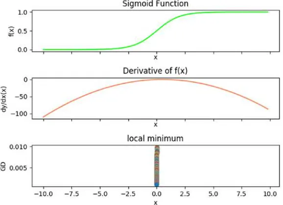
Sigmoid Function Minimization (and Maximization) ��104

Euclidean Distance Minimization Controlling for Step Size ��109

Stabilizing Euclidean Distance Minimization with

Monte Carlo Simulation ��112

Substituting a NumPy Method to Hasten Euclidean

Distance Minimization ��115

Stochastic Gradient Descent Minimization and Maximization ��118

Chapter 5: Working with Data 129

One-Dimensional Data Example ��129

Two-Dimensional Data Example ��132

Data Correlation and Basic Statistics ��135

Pandas Correlation and Heat Map Examples ��138

Various Visualization Examples ��141

Cleaning a CSV File with Pandas and JSON ��146

Slicing and Dicing ��148

Data Cubes ��149

(7)

Chapter 6: Exploring Data 167

Heat Maps ��167

Principal Component Analysis ��170

Speed Simulation ��179

Big Data ��182

Twitter ��201

Web Scraping ��205

(8)

About the Author

David Paper is a full professor at Utah State University in the Management Information Systems department. His book Web Programming for Business: PHP Object-Oriented Programming with Oracle was published in 2015 by Routledge. He also has over 70 publications in refereed journals such as Organizational Research Methods, Communications of the ACM, Information & Management, Information Resource Management Journal, Communications of the AIS, Journal of Information Technology Case and Application Research, and Long Range Planning. He has also served on several editorial boards in various capacities, including associate editor. Besides growing up in family businesses, Dr. Paper has worked for Texas Instruments, DLS, Inc., and the Phoenix Small Business Administration. He has performed IS consulting work for IBM, AT&T, Octel, Utah

(9)

About the Technical Reviewer

(10)

Acknowledgments

(11)

Introduction

Data science is an interdisciplinary field encompassing scientific methods, processes, and systems to extract knowledge or insights from data in various forms, either structured or unstructured. It draws principles from mathematics, statistics, information science, computer science, machine learning, visualization, data mining, and predictive analytics. However, it is fundamentally grounded in mathematics.

This book explains and applies the fundamentals of data science crucial for technical professionals such as DBAs and developers who are making career moves toward practicing data science. It is an example-driven book providing complete Python coding examples to complement and clarify data science concepts, and enrich the learning experience. Coding examples include visualizations whenever appropriate. The book is a necessary precursor to applying and implementing machine learning algorithms, because it introduces the reader to foundational principles of the science of data.

(12)

Data Science Fundamentals by Example is an excellent starting point for those interested in pursuing a career in data science. Like any science, the fundamentals of data science are prerequisite to competency. Without proficiency in mathematics, statistics, data manipulation, and coding, the path to success is “rocky” at best. The coding examples in this book are concise, accurate, and complete, and perfectly complement the data science concepts introduced.

The book is organized into six chapters. Chapter 1 introduces the programming fundamentals with “Python” necessary to work with, transform, and process data for data science applications. Chapter 2 introduces Monte Carlo simulation for decision making, and data

distributions for statistical processing. Chapter 3 introduces linear algebra applied with vectors and matrices. Chapter 4 introduces the gradient descent algorithm that minimizes (or maximizes) functions, which is very important because most data science problems are optimization problems. Chapter 5 focuses on munging, cleaning, and transforming data for solving data science problems. Chapter 6 focusing on exploring data by dimensionality reduction, web scraping, and working with large data sets efficiently.

Python programming code for all coding examples and data files are available for viewing and download through Apress at www.apress.com/ 9781484235966. Specific linking instructions are included on the

copyright pages of the book.

(13)

Python Fundamentals

Python has several features that make it well suited for learning and doing data science. It’s free, relatively simple to code, easy to understand, and has many useful libraries to facilitate data science problem solving. It also allows quick prototyping of virtually any data science scenario and demonstration of data science concepts in a clear, easy to understand manner.

The goal of this chapter is not to teach Python as a whole, but present, explain, and clarify fundamental features of the language (such as logic, data structures, and libraries) that help prototype, apply, and/or solve data science problems.

Python fundamentals are covered with a wide spectrum of activities with associated coding examples as follows:

1. functions and strings

2. lists, tuples, and dictionaries

3. reading and writing data

4. list comprehension

5. generators

6. data randomization

7. MongoDB and JSON

8. visualization

(14)

either custom or built-in. Custom are created by the programmer, while built-in are part of the language. Strings are very popular types enclosed in either single or double quotes.

The following code example defines custom functions and uses built-in ones:

# hash symbol allows single-line comments '''

(15)

print ('\nstring', '"' + string + '" has', len(string), 'characters')

str_ls = string.split()

print ('split string:', str_ls)

print ('joined list:', ' '.join(str_ls))

Output:

(16)

Lists, Tuples, and Dictionaries

Lists are ordered collections with comma-separated values between square brackets. Indices start at 0 (zero). List items need not be of the same type and can be sliced, concatenated, and manipulated in many ways.

The following code example creates a list, manipulates and slices it, creates a new list and adds elements to it from another list, and creates a matrix from two lists:

import numpy as np

if __name__ == "__main__":

ls = ['orange', 'banana', 10, 'leaf', 77.009, 'tree', 'cat'] print ('list length:', len(ls), 'items')

print ('cat count:', ls.count('cat'), ',', 'cat index:', ls.index('cat'))

print ('\nmanipulate list:') cat = ls.pop(6)

print ('cat:', cat, ', list:', ls) ls.insert(0, 'cat')

(17)

ls.pop() print (ls)

print ('\nslice list:')

print ('1st 3 elements:', ls[:3]) print ('last 3 elements:', ls[3:])

print ('start at 2nd to index 5:', ls[1:5])

print ('start 3 from end to end of list:', ls[-3:])

print ('start from 2nd to next to end of list:', ls[1:-1]) print ('\ncreate new list from another list:')

print ('list:', ls) fruit = ['orange']

more_fruit = ['apple', 'kiwi', 'pear'] fruit.append(more_fruit)

print ('appended:', fruit) fruit.pop(1)

fruit.extend(more_fruit) print ('extended:', fruit) a, b = fruit[2], fruit[1] print ('slices:', a, b)

print ('\ncreate matrix from two lists:') matrix = np.array([ls, fruit])

print (matrix)

(18)

Output:

(19)

Second, print the last three elements with ls[3:]. Third, print starting with the 2nd element to elements with indices up to 5 with ls[1:5]. Fourth, print starting three elements from the end to the end with ls[-3:]. Fifth, print starting from the 2nd element to next to the last element with ls[1:-1]. The code continues by creating a new list from another. First, create fruit with one element. Second append list more_fruit to fruit. Notice that append adds list more_fruit as the 2nd element of fruit, which may not be what you want. So, third, pop 2nd element of fruit and extend more_fruit to fruit. Function extend() unravels a list before it adds it. This way, fruit now has four elements. Fourth, assign 3rd element to a and 2nd element to b and print slices. Python allows assignment of multiple variables on one line, which is very convenient and concise. The code ends by creating a matrix from two lists—ls and fruit—and printing it. A Python matrix is a two-dimensional (2-D) array consisting of rows and columns, where each row is a list.

A tuple is a sequence of immutable Python objects enclosed by

parentheses. Unlike lists, tuples cannot be changed. Tuples are convenient with functions that return multiple values.

The following code example creates a tuple, slices it, creates a list, and creates a matrix from tuple and list:

if __name__ == "__main__":

tup = ('orange', 'banana', 'grape', 'apple', 'grape') print ('tuple length:', len(tup))

print ('grape count:', tup.count('grape')) print ('\nslice tuple:')

(20)

print ('start from 2nd to next to end of tuple:', tup[1:-1]) print ('\ncreate list and create matrix from it and tuple:') fruit = ['pear', 'grapefruit', 'cantaloupe', 'kiwi', 'plum'] matrix = np.array([tup, fruit])

print (matrix)

Output:

The code begins by importing NumPy. The main block begins by creating tuple tup, printing its length, number of elements (items), number of grape elements, and index of grape. The code continues by slicing tup. First, print the 1st three elements with tup[:3]. Second, print the last three elements with tup[3:]. Third, print starting with the 2nd element to elements with indices up to 5 with tup[1:5]. Fourth, print starting three elements from the end to the end with tup[-3:]. Fifth, print starting from the 2nd element to next to the last element with tup[1:-1]. The code

(21)

The following code example creates a dictionary, deletes an element, adds an element, creates a list of dictionary elements, and traverses the list:

if __name__ == "__main__":

audio = {'amp':'Linn', 'preamp':'Luxman', 'speakers':'Energy', 'ic':'Crystal Ultra', 'pc':'JPS', 'power':'Equi-Tech', 'sp':'Crystal Ultra', 'cdp':'Nagra', 'up':'Esoteric'} del audio['up']

print ('dict "deleted" element;') print (audio, '\n')

print ('dict "added" element;') audio['up'] = 'Oppo'

print (audio, '\n')

print ('universal player:', audio['up'], '\n') dict_ls = [audio]

video = {'tv':'LG 65C7 OLED', 'stp':'DISH', 'HDMI':'DH Labs', 'cable' : 'coax'}

print ('list of dict elements;') dict_ls.append(video)

for i, row in enumerate(dict_ls): print ('row', i, ':')

print (row)

(22)

The main block begins by creating dictionary audio with several elements. It continues by deleting an element with key up and value Esoteric, and displaying. Next, a new element with key up and element Oppo is added back and displayed. The next part creates a list with dictionary audio, creates dictionary video, and adds the new dictionary to the list. The final part uses a for loop to traverse the dictionary list and display the two dictionaries. A very useful function that can be used with a loop statement is enumerate(). It adds a counter to an iterable. An iterable is an object that can be iterated. Function enumerate() is very useful because a counter is automatically created and incremented, which means less code.

Reading and Writing Data

The ability to read and write data is fundamental to any data science endeavor. All data files are available on the website. The most basic types of data are text and CSV (Comma Separated Values). So, this is where we will start.

The following code example reads a text file and cleans it for processing. It then reads the precleansed text file, saves it as a CSV file, reads the CSV file, converts it to a list of OrderedDict elements, and converts this list to a list of regular dictionary elements.

(23)

writer = csv.writer(csv_file)

(24)

r_dict = read_dict(csv_f, headers) dict_ls = []

print ('\ncsv to ordered dict sample:') for i, row in enumerate(r_dict):

r = od_to_d(row) dict_ls.append(r) if i < 3:

print (row)

print ('\nlist of dictionary elements sample:') for i, row in enumerate(dict_ls):

if i < 3: print (row)

Output:

(25)

to define and create a list in Python. List comprehension is covered later in the next section. Function conv_csv() converts a text to a CSV file and saves it to disk. Function read_csv() reads a CSV file and returns it as a list. Function read_dict() reads a CSV file and returns a list of OrderedDict elements. An OrderedDict is a dictionary subclass that remembers the order in which its contents are added, whereas a regular dictionary doesn’t track insertion order. Finally, function od_to_d() converts an OrderedDict element to a regular dictionary element. Working with a regular dictionary element is much more intuitive in my opinion. The main block begins by reading a text file and cleaning it for processing. However, no processing is done with this cleansed file in the code. It is only included in case you want to know how to accomplish this task. The code continues by converting a text file to CSV, which is saved to disk. The CSV file is then read from disk and a few records are displayed. Next, a headers list is created to store keys for a dictionary yet to be created. List dict_ls is created to hold dictionary elements. The code continues by creating an OrderedDict list r_dict. The OrderedDict list is then iterated so that each element can be converted to a regular dictionary element and appended to dict_ls. A few records are displayed during iteration. Finally, dict_ls is iterated and a few records are displayed. I highly recommend that you take some time to familiarize yourself with these data structures, as they are used extensively in data science application.

List Comprehension

(26)

The logic strips extraneous characters from string in iterable d. In this case, d is a list of strings.

The following code example converts miles to kilometers, manipulates pets, and calculates bonuses with list comprehension:

if __name__ == "__main__":

miles = [100, 10, 9.5, 1000, 30]

kilometers = [x * 1.60934 for x in miles] print ('miles to kilometers:')

(27)

d[row] = bonus[i] print (d, '\n')

print ('{:<5} {:<5}'.format('emp', 'bonus')) for k, y in d.items():

print ('{:<5} {:>6}'.format(k, y))

Output:

(28)

with up to eight characters. Finally, each string for km is right justified ({:>2}) with up to two characters. This may seem a bit complicated at first, but it is really quite logical (and elegant) once you get used to it. The main block continues by creating pet and pets lists. The pets list is created with list comprehension, which makes a pet plural if it is not a fish. I advise you to study this list comprehension before you go forward, because they just get more complex. The code continues by creating a subset list with list comprehension, which only includes dogs and cats. The next part creates two lists—sales and bonus. Bonus is created with list comprehension that calculates bonus for each sales value. If sales are less than 10,000, no bonus is paid. If sales are between 10,000 and 20,000 (inclusive), the bonus is 2% of sales. Finally, if sales if greater than 20,000, the bonus is 3% of sales. At first I was confused with this list comprehension but it makes sense to me now. So, try some of your own and you will get the gist of it. The final part creates a people list to associate with each sales value, continues by creating a dictionary to hold bonus for each person, and ends by iterating dictionary elements. The formatting is quite elegant. The header left justifies emp and bonus properly. Each item is formatted so that the person is left justified with up to five characters ({:<5}) and the bonus is right justified with up to six characters ({:>6}).

Generators

(29)

The following code example reads a CSV file and creates a list of OrderedDict elements. It then converts the list elements into regular dictionary elements. The code continues by simulating times for list comprehension, generator comprehension, and generators. During simulation, a list of times for each is created. Simulation is the imitation of a real-world process or system over time, and it is used extensively in data science.

import csv, time, numpy as np

def read_dict(f, h):

(30)

def gen(d): dict_ls = conv_reg_dict(r_dict) n = 1000

(31)

print ('generator comprehension:')

print (gc_ls, 'times faster than list comprehension\n') print ('generator:')

print (g_ls, 'times faster than list comprehension')

Output:

(32)

a list of those runtimes for each. The 2nd simulation calculates 1,000 runtimes by traversing the dictionary list for a generator, and returns a list of those runtimes. The code concludes by calculating the average runtime for each of the three techniques—list comprehension, generator comprehension, and generators—and comparing those averages.

The simulations verify that generator comprehension is more than ten times, and generators are more than eight times faster than list comprehension (runtimes will vary based on your PC). This makes sense because list comprehension stores all data in memory, while generators evaluate (lazily) as data is needed. Naturally, the speed advantage of generators becomes more important with big data sets. Without

simulation, runtimes cannot_{be verified because we are randomly getting}

internal system clock times.

Data Randomization

A stochastic process is a family of random variables from some probability space into a state space (whew!). Simply, it is a random process through time. Data randomization is the process of selecting values from a sample in an unpredictable manner with the goal of simulating reality. Simulation allows application of data randomization in data science. The previous section demonstrated how simulation can be used to realistically compare iterables (list comprehension, generator comprehension, and generators).

In Python, pseudorandom numbers are used to simulate data randomness (reality). They are not truly random because the 1st

generation has no previous number. We have to provide a seed (or random seed) to initialize a pseudorandom number generator. The random

library implements pseudorandom number generators for various data distributions, and random.seed() is used to generate the initial

(33)

The following code example reads a CSV file and converts it to a list of regular dictionary elements. The code continues by creating a random number used to retrieve a random element from the list. Next, a generator of three randomly selected elements is created and displayed. The code continues by displaying three randomly shuffled elements from the list. The next section of code deterministically seeds the random number generator, which means that all generated random numbers will be the same based on the seed. So, the elements displayed will always be the same ones unless the seed is changed. The code then uses the system’s time to nondeterministically generate random numbers and display those three elements. Next, nondeterministic random numbers are generated by another method and those three elements are displayed. The final part creates a names list so random choice and sampling methods can be used to display elements.

import csv, random, time

input_file = csv.DictReader(open(f), fieldnames=h) return (input_file)

def conv_reg_dict(d):

return [dict(x) for x in d]

def r_inds(ls, n): length = len(ls) - 1

yield [random.randrange(length) for _ in range(n)]

def get_slice(ls, n): return ls[:n]

(34)

if __name__ == '__main__': f = 'data/names.csv'

headers = ['first', 'last'] r_dict = read_dict(f, headers) dict_ls = conv_reg_dict(r_dict) n = len(dict_ls)

r = random.randrange(0, n-1)

print ('randomly selected index:', r)

print ('randomly selected element:', dict_ls[r]) elements = 3

generator = next(r_inds(dict_ls, elements)) p_line()

print (elements, 'randomly generated indicies:', generator) print (elements, 'elements based on indicies:')

for row in generator: print (dict_ls[row]) x = [[i] for i in range(n-1)] random.shuffle(x)

p_line()

print ('1st', elements, 'shuffled elements:') ind = get_slice(x, elements)

for row in ind:

print (dict_ls[row[0]]) seed = 1

random_seed = random.seed(seed) rs1 = random.randrange(0, n-1) p_line()

print ('deterministic seed', str(seed) + ':', rs1) print ('corresponding element:', dict_ls[rs1]) t = time.time()

(35)

rs2 = random.randrange(0, n-1) p_line()

print ('non-deterministic time seed', str(t) + ' index:', rs2) print ('corresponding element:', dict_ls[rs2], '\n')

print (elements, 'random elements seeded with time:') for i in range(elements):

r = random.randint(0, n-1) print (dict_ls[r], r) random_seed = random.seed() rs3 = random.randrange(0, n-1) p_line()

print ('non-deterministic auto seed:', rs3)

print ('corresponding element:', dict_ls[rs3], '\n') print (elements, 'random elements auto seed:') for i in range(elements):

print (elements, 'names with "random.choice()":') for row in range(elements):

print (random.choice(names)) p_line()

(36)

Output:

The code begins by importing csv, random, and time libraries. Functions read_dict() and conv_reg_dict() have already been explained. Function r_inds() generates a random list of n elements from the

(37)

lists begin at index zero. Function get_slice() creates a randomly shuffled list of n elements from the dictionary list. Function p_line() prints a blank line. The main block begins by reading a CSV file and converting it into a list of regular dictionary elements. The code continues by creating a random number with random.randrange() based on the number of indices from the dictionary list, and displays the index and associated dictionary element. Next, a generator is created and populated with three randomly determined elements. The indices and associated elements are printed from the generator. The next part of the code randomly shuffles the indicies and puts them in list x. An index value is created by slicing three random elements based on the shuffled indices stored in list x. The three elements are then displayed. The code continues by creating a deterministic random seed using a fixed number (seed) in the function. So, the random number generated by this seed will be the same each time the program is run. This means that the dictionary element displayed will be also be the same. Next, two methods for creating nondeterministic random numbers are presented—random.seed(t) and random.seed()— where t varies by system time and using no parameter automatically varies random numbers. Randomly generated elements are displayed for each method. The final part of the code creates a list of names to hold just first and last names, so random.choice() and random.sample() can be used.

MongoDB and JSON

(38)

a document is conceptually like a row. JSON is a lightweight

data-interchange format that is easy for humans to read and write. It is also easy for machines to parse and generate.

Database queries from MongoDB are handled by PyMongo. PyMongo is a Python distribution containing tools for working with MongoDB. It is the most efficient tool for working with MongoDB using the utilities of Python. PyMongo was created to leverage the advantages of Python as a programming language and MongoDB as a database. The pymongo library is a native driver for MongoDB, which means it is it is built into Python language. Since it is native, the pymongo library is automatically available (doesn’t have to be imported into the code).

The following code example reads a CSV file and converts it to a list of regular dictionary elements. The code continues by creating a JSON file from the dictionary list and saving it to disk. Next, the code connects to MongoDB and inserts the JSON data. The final part of the code manipulates data from the MongoDB database. First, all data in the database is queried and a few records are displayed. Second, the database is rewound. Rewind sets the pointer to back to the 1st database record. Finally, various queries are performed.

import json, csv, sys, os

sys.path.append(os.getcwd()+'/classes') import conn

input_file = csv.DictReader(open(f), fieldnames=h) return (input_file)

def conv_reg_dict(d):

(39)

(40)

if i < n: print (row)

print ('\nquery 1st', n, 'names') first_n = names.find().limit(n) for row in first_n:

query_1st_in_list = names.find( {'first':{'$in':[fnames[0]]}}) for row in query_1st_in_list:

print (row)

print ('\nquery Ella or Lou:')

query_1st = names.find( {'first':{'$in':fnames}} ) for row in query_1st:

print (row)

print ('\nquery Lou Pole:')

query_and = names.find( {'first':fnames[1], 'last':lnames[1]} ) for row in query_and:

print (row)

print ('\nquery first name Ella or last name Pole:') query_or = names.find( {'$or':[{'first':fnames[0]},

(41)

for row in query_or: print (row) pattern = '^Sch'

print ('\nquery regex pattern:')

query_like = names.find( {'last':{'$regex':pattern}} ) for row in query_like:

print (row) pid = names.count()

doc = {'_id':pid, 'first':'Wendy', 'last':'Day'} names.insert_one(doc)

print ('\ndisplay added document:') q_added = names.find({'first':'Wendy'}) print (q_added.next())

print ('\nquery last n documents:') q_n = names.find().skip((pid-n)+1) for _ in range(n):

print (q_n.next())

Class conn:

class conn:

from pymongo import MongoClient

client = MongoClient('localhost', port=27017) def __init__(self, dbname):

self.db = conn.client[dbname] def getDB(self):

(42)

(43)

(44)

Sch. A regular expression is a sequence of characters that define a search pattern. Finally, add a new document, display it, and display the last three documents in the collection.

Visualization

Visualization is the process of representing data graphically and leveraging these representations to gain insight into the data. Visualization is one of the most important skills in data science because it facilitates the way we process large amounts of complex data.

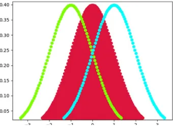
The following code example creates and plots a normally distributed set of data. It then shifts data to the left (and plots) and shifts data to the right (and plots). A normal distribution is a probability distribution that is symmetrical about the mean, and is very important to data science because it is an excellent model of how events naturally occur in reality.

import matplotlib.pyplot as plt from scipy.stats import norm import numpy as np

if __name__ == '__main__':

x = np.linspace(norm.ppf(0.01), norm.ppf(0.99), num=100) x_left = x - 1

x_right = x + 1 y = norm.pdf(x) plt.ylim(0.02, 0.41)

(45)

Output:

(46)

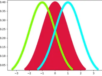
On the 1st line of the main block in the linespace() function, increase the number of data points from num = 100 to num = 1000 and see what happens. The result is a smoothing of the normal distribution, because more data provides a more realistic picture of the natural world.

Output:

Smoothing works (Figure 1-2) because a normal distribution consists of continuous random variables. A continuous random variable is a random variable with a set of infinite and uncountable values. So, more data creates more predictive realism. Since we cannot add infinite data, we work with as much data as we can. The tradeoff is more data increases computer processing resources and execution time. Data scientists must thereby weigh this tradeoff when conducting their tradecraft.

(47)

Monte Carlo

Simulation and

Density Functions

Monte Carlo simulation (MCS) applies repeated random sampling (randomness) to obtain numerical results for deterministic problem solving. It is widely used in optimization, numerical integration, and risk-based decision making. Probability and cumulative density functions are statistical measures that apply probability distributions for random variables, and can be used in conjunction with MCS to solve deterministic problem.

Note Reader can refer to the download source code file to see color

figs in this chapter.

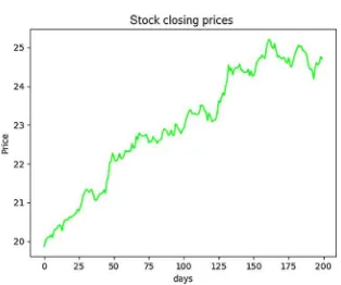
Stock Simulations

(48)

import matplotlib.pyplot as plt, numpy as np from scipy import stats

def cum_price(p, d, m, s): data = []

for d in range(d):

prob = stats.norm.rvs(loc=m, scale=s) price = (p * prob)

data.append(price) p = price

return data

if __name__ == "__main__":

stk_price, days, mean, s = 20, 200, 1.001, 0.005 data = cum_price(stk_price, days, mean, s) plt.plot(data, color='lime')

plt.ylabel('Price') plt.xlabel('days')

(49)

Output:

The code begins by importing matplotlib, numpy, and scipy libraries. It continues with function cum_price(), which generates 200 normally distributed random numbers (one for each day) with norm_rvs(). Data randomness is key. The main block creates the variables. Mean is set a bit over 1 and standard deviation (s) at a very small number to generate a slowly increasing stock price. Mean (mu) is the average change in value. Standard deviation is the variation or dispersion in the data. With s of 0.005, our data has very little variation. That is, the numbers in our data set are very close to each other. Remember that this is not a real scenario! The

(50)

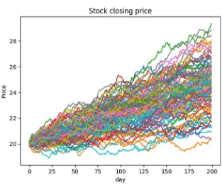
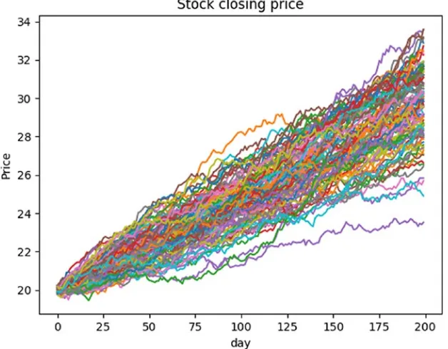
The next example adds MCS into the mix with a while loop that iterates 100 times:

import matplotlib.pyplot as plt, numpy as np from scipy import stats

def cum_price(p, d, m, s): data = []

for d in range(d):

prob = stats.norm.rvs(loc=m, scale=s) price = (p * prob)

data.append(price) p = price

return data

if __name__ == "__main__":

stk_price, days, mu, sigma = 20, 200, 1.001, 0.005 x = 0

while x < 100:

data = cum_price(stk_price, days, mu, sigma) plt.plot(data)

x += 1

plt.ylabel('Price') plt.xlabel('day')

(51)

Output:

The while loop allows us to visualize (as shown in Figure 2-2) 100 possible stock price outcomes over 200 days. Notice that mu (mean) and sigma (standard deviation) are used. This example demonstrates the power of MCS for decision making.

(52)

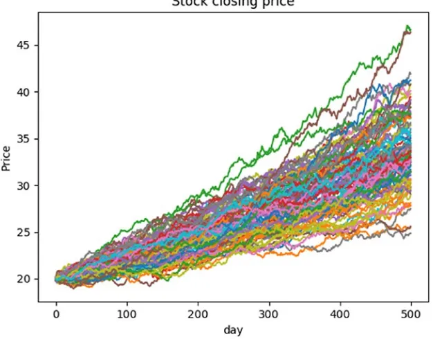
What-If Analysis

What-If analysis changes values in an algorithm to see how they impact outcomes. Be sure to only change one variable at a time, otherwise you won’t know which caused the change. In the previous example, what if we change days to 500 while keeping all else constant (the same)? Plotting this change results in the following (Figure 2-3):

(53)

Figure 2-4.

What-If analysis for mu = 1.002

(54)

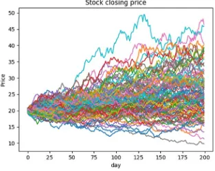
Changing sigma to 0.02 results in more variation as follows (Figure 2- 5):

Product Demand Simulation

A discrete probability is the probability of each discrete random value occurring in a sample space or population. A random variable assumes different values determined by chance. A discrete random variable can only assume a countable number of values. In contrast, a continuous random variable can assume an uncountable number of values in a line interval such as a normal distribution.

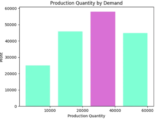
In the code example, demand for a fictitious product is predicted by four discrete probability outcomes: 10% that random variable is 10,000 units, 35% that random variable is 20,000 units, 30% that random variable is 40,000 units, and 25% that random variable is 60,000 units. Simply,

(55)

10% of the time demand is 10,000, 35% of the time demand is 20,000, 30% of the time demand is 40,000, and 25% of the time demand is 60,000. Discrete outcomes must total 100%. The code runs MCS on a production algorithm that determines profit for each discrete outcome, and plots the results.

import matplotlib.pyplot as plt, numpy as np

def demand():

def production(demand, units, price, unit_cost, disposal): units_sold = min(units, demand)

revenue = units_sold * price

(56)

def mcs(x, n, units, price, unit_cost, disposal):

profit_10 = mcs(x, n, units[0], price, unit_cost, disposal) avg_p.append(np.mean(profit_10))

print ('Profit for {:,.0f}'.format(units[0]), 'units: ${:,.2f}'.format(np.mean(profit_10)))

profit_20 = mcs(x, n, units[1], price, unit_cost, disposal) avg_p.append(np.mean(np.mean(profit_20)))

profit_40 = mcs(x, n, units[2], price, unit_cost, disposal) avg_p.append(np.mean(profit_40))

(57)

print ('Profit for {:,.0f}'.format(units[3]), 'units: ${:,.2f}'.format(np.mean(profit_60))) labels = ['10000','20000','40000','60000']

pos = np.arange(len(labels))

width = 0.75 # set less than 1.0 for spaces between bins plt.figure(2)

ax = plt.axes()

ax.set_xticks(pos + (width / 2)) ax.set_xticklabels(labels)

barlist = plt.bar(pos, avg_p, width, color='aquamarine') barlist[max_bar(avg_p)].set_color('orchid')

plt.ylabel('Profit')

plt.xlabel('Production Quantity')

plt.title('Production Quantity by Demand') plt.show()

(58)

The code begins by importing matplotlib and numpy libraries. It continues with four functions. Function demand() begins by randomly generating a uniformly distributed probability. It continues by returning one of the four discrete probability outcomes established by the problem we wish to solve. Function production() returns profit based on an algorithm that I devised. Keep in mind that any profit-base algorithm can be substitued, which illuminates the incredible flexibility of MCS. Function mcs() runs the simulation 10,000 times. Increasing the number of runs provides better prediction accuracy with costs being more computer processing resources and runtime. Function max_bar() establishes the highest bar in the bar chart for better illumination. The main block begins by simulating profit for each discrete probability outcome, and printing and visualizing results. MCS predicts that production quantity of 40,000 units yields the highest profit, as shown in Figure 2-6.

(59)

Increasing the number of MCS simulations results in a more

accurate prediction of reality because it is based on stochastic reasoning (data randomization). You can also substitute any discrete probability distribution based on your problem-solving needs with this code structure. As alluded to earlier, you can use any algorithm you wish to predict with MCS, making it an incredibly flexible tool for data scientists.

We can further enhance accuracy by running an MCS on an MCS. The code example uses the same algorithm and process as before, but adds an MCS on the original MCS to get a more accurate prediction:

def demand():

def production(demand, units, price, unit_cost, disposal): units_sold = min(units, demand)

revenue = units_sold * price total_cost = units * unit_cost units_not_sold = units - demand if units_not_sold > 0:

(60)

else:

disposal_cost = 0

profit = revenue - total_cost - disposal_cost return profit

def mcs(x, n, units, price, unit_cost, disposal): profit = []

(61)

avg_profit = np.mean(profit_60)

avg_ls.append({'p10':np.mean(profit_10), 'p20':np.mean(profit_20), 'p40':np.mean(profit_40), 'p60':np.mean(profit_60)}) y += 1

mcs_p10, mcs_p20, mcs_p40, mcs_p60 = [], [], [], [] for row in avg_ls:

mcs_p10.append(row['p10']) mcs_p20.append(row['p20']) mcs_p40.append(row['p40']) mcs_p60.append(row['p60']) display(np.mean(mcs_p10), 0) display(np.mean(mcs_p20), 1) display(np.mean(mcs_p40), 2) display(np.mean(mcs_p60), 3)

Output:

(62)

Randomness Using Probability

and Cumulative Density Functions

Randomness masquerades as reality (the natural world) in data science, since the future cannot be predicted. That is, randomization is the way data scientists simulate reality. More data means better accuracy and prediction (more realism). It plays a key role in discrete event simulation and deterministic problem solving. Randomization is used in many fields such as statistics, MCS, cryptography, statistics, medicine, and science.

The density of a continuous random variable is its probability density function (PDF). PDF is the probability that a random variable has the value x, where x is a point within the interval of a sample. This probability is determined by the integral of the random variable’s PDF over the range (interval) of the sample. That is, the probability is given by the area under the density function, but above the horizontal axis and between the lowest and highest values of range. An integral (integration) is a mathematical object that can be interpreted as an area under a normal distribution curve. A cumulative distribution function (CDF) is the probability that a random variable has a value less than or equal to x. That is, CDF accumulates all of the probabilities less than or equal to x. The percent point function (PPF) is the inverse of the CDF. It is commonly referred to as the inverse cumulative distribution function (ICDF). ICDF is very useful in data science because it is the actual value associated with an area under the PDF. Please refer to www.itl.nist.gov/div898/handbook/eda/ section3/eda362.htm for an excellent explanation of density functions.

(63)

being integrated in either a definite or indefinite integral. The fundamental theorem of calculus relates the evaluation of definitive integrals to

indefinite integrals. The only reason I include this information here is to emphasize the importance of calculus to data science. Another aspect of calculus important to data science, “gradient descent,” is presented later in Chapter 4.

Although theoretical explanations are invaluable, they may not be intuitive. A great way to better understand these concepts is to look at an example.

In the code example, 2-D charts are created for PDF, CDF, and ICDF (PPF). The idea of a colormap is included in the example. A colormap is a lookup table specifying the colors to be used in rendering palettized image. A palettized image is one that is efficiently encoded by mapping its pixels to a palette containing only those colors that are actually present in the image. The matplotlib library includes a myriad of colormaps. Please refer to https://matplotlib.org/examples/color/colormaps_reference.html

x = np.linspace(norm.ppf(0.01), norm.ppf(0.99), num=1000) y1 = norm.pdf(x)

plt.figure('PDF')

plt.xlim(x.min()-.1, x.max()+0.1) plt.ylim(y1.min(), y1.max()+0.01) plt.xlabel('x')

(64)

plt.fill_between(x, y1, color='thistle') plt.show()

plt.close('PDF') plt.figure('CDF') plt.xlabel('x')

plt.ylabel('Probability') plt.title('Normal CDF') y2 = norm.cdf(x)

plt.scatter(x, y2, c=x, cmap='jet') plt.show()

plt.close('CDF') plt.figure('ICDF')

plt.xlabel('Probability') plt.ylabel('x')

plt.title('Normal ICDF (PPF)') y3 = norm.ppf(x)

plt.scatter(x, y3, c=x, cmap='jet') plt.show()

(65)

(66)

The code begins by importing three libraries—matplotlib, scipy, and numpy. The main block begins by creating a sequence of 1,000 x values between 0.01 and 0.99 (because probabilities must fall between 0 and 1). Next, a sequence of PDF y values is created based on the x values. The code continues by plotting the resultant PDF shown in Figure 2-7. Next, a sequence of CDF (Figure 2-8) and ICDF (Figure 2-9) values are created and plotted. From the visualization, it is easier to see that the PDF represents all of the possible x values (probabilities) that exist under the normal distribution. It is also easier to visualize the CDF because it represents the accumulation of all the possible probabilities. Finally, the ICDF is easier to understand through visualization (see Figure 2-9) because the x-axis represents probabilities, while the y-axis represents the actual value associated with those probabilities.

(67)

Let’s apply ICDF. Suppose you are a data scientist at Apple and your boss asks you to determine Apple iPhone 8 failure rates so she can develop a mockup presentation for her superiors. For this hypothetical example, your boss expects four calculations: time it takes 5% of phones to fail, time interval (range) where 95% of phones fail, time where 5% of phones survive (don’t fail), and time interval where 95% of phones survive. In all cases, report time in hours. From data exploration, you ascertain average (mu) failure time is 1,000 hours and standard deviation (sigma) is 300 hours.

The code example calculates ICDF for the four scenarios and displays the results in an easy to understand format for your boss:

from scipy.stats import norm import numpy as np

def np_rstrip(v):

return np.char.rstrip(v.astype(str), '.0')

def transform(t):

one, two = round(t[0]), round(t[1]) return (np_rstrip(one), np_rstrip(two))

if __name__ == "__main__": mu, sigma = 1000, 300

print ('Expected failure rates:')

fail = np_rstrip(round(norm.ppf(0.05, loc=mu, scale=sigma))) print ('5% fail within', fail, 'hours')

fail_range = norm.interval(0.95, loc=mu, scale=sigma) lo, hi = transform(fail_range)

print ('95% fail between', lo, 'and', hi, end=' ') print ('hours of usage')

(68)

last_range = norm.interval(0.05, loc=mu, scale=sigma) lo, hi = transform(last_range)

print ('95% survive between', lo, 'and', hi, 'hours of usage')

Output:

The code example begins by importing scipy and numpy libraries. It continues with two functions. Function np_rstrip() converts numpy float to string and removes extraneous characters. Function transform() rounds and returns a tuple. Both are just used to round numbers to no decimal places to make it user-friendly for your fictitious boss. The main block begins by initializing mu and sigma to 1,000 (failures) and 300 (variates). That is, on average, our smartphones fail within 1,000 hours, and failures vary between 700 and 1,300 hours. Next, find the ICDF value for a 5% failure rate and an interval where 95% fail with norm.ppf(). So, 5% of all phones are expected to fail within 507 hours, while 95% fail between 412 and 1,588 hours of usage. Next, find the ICDF value for a 5% survival rate and an interval where 95% survive. So, 5% of all phones survive up to 1,493 hours, while 95% survive between 981 and 1,019 hours of usage.

(69)

Let’s try What-if analysis. What if we reduce error rate (sigma) from 300 to 30?

Now, 5% of all phones are expected to fail within 951 hours, while 95% fail between 941 and 1,059 hours of usage. And, 5% of all phones survive up to 1,049 hours, while 95% survive between 998 and 1,002 hours of usage. What does this mean? Less variation (error) shows that values are much closer to the average for both failure and survival rates. This makes sense because variation is calculated from a mean of 1,000.

Let’s shift to a simulation example. Suppose your boss asks you to find the optimal monthly order quantity for a type of car given that demand is normally distributed (it must, because PDF is based on this assumption), average demand (mu) is 200, and variation (sigma) is 30. Each car costs $25,000, sells for $45,000, and half of the cars not sold at full price can be sold for $30,000. Like other MCS experiments, you can modify the profit algorithm to enhance realism. By suppliers, you are limited to order quantities of 160, 180, 200, 220, 240, 260, or 280.

MCS is used to find the profit for each order based on the information provided. Demand is generated randomly for each iteration of the

simulation. Profit calculations by order are automated by running MCS for each order.

(70)

if __name__ == "__main__":

max_profit = max(profit_ls) profit_np = np.array(profit_ls)

max_ind = np.where(profit_np == profit_np.max())

(71)

'for order', orders[int(max_ind[0])]) barlist = plt.bar(orders, profit_ls, width=15, color='thistle')

barlist[int(max_ind[0])].set_color('lime') plt.title('Profits by Order Quantity') plt.xlabel('orders')

plt.ylabel('profit') plt.tight_layout() plt.show()

(72)

The code begins by importing numpy and matplotlib. It continues with a function (str_int()) that converts a string to float. The main block begins by initializing orders, mu, sigma, n, cost, price, discount, and list of profits by order. It continues by looping through each order quantity and running MCS with 10,000 iterations. A randomly generated demand probability is used to calculate profit for each iteration of the simulation. The technique for calculating profit is pretty simple, but you can substitute your own algorithm. You can also modify any of the given information based on your own data. After calculating profit for each order through MCS, the code continues by finding the order quantity with the highest profit. Finally, the code generates a bar chart to illuminate results though visualization shown in Figure 2-10.

(73)

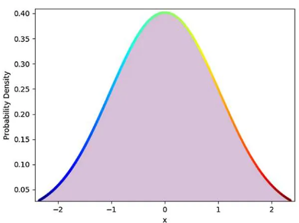
The final code example creates a PDF visualization:

import matplotlib.pyplot as plt, numpy as np from scipy.stats import norm

if __name__ == '__main__': n = 100

x = np.linspace(norm.ppf(0.01), norm.ppf(0.99), num=n) y = norm.pdf(x)

dic = {}

for i, row in enumerate(y):

dic[x[i]] = [np.random.uniform(0, row) for _ in range(n)] xs = []

ys = []

for key, vals in dic.items(): for y in vals:

xs.append(key) ys.append(y) plt.xlim(min(xs), max(xs)) plt.ylim(0, max(ys)+0.02) plt.title('Normal PDF') plt.xlabel('x')

plt.ylabel('Probability Density')

(74)

Output:

The code begins by importing matplotlib, numpy, and scipy libraries. The main block begins by initializing the number of points you wish to plot, PDF x and y values, and a dictionary. To plot all PDF probabilities, a set of randomly generated values for each point on the x-axis is created. To accomplish this task, the code assigns 100 (n = 100) values to x from 0.01 to 0.99. It continues by assigning 100 PDF values to y. Next, a dictionary element is populated by a (key, value) pair consisting of each x value as key and a list of 100 (n = 100) randomly generated numbers between 0 and pdf(x) as value associated with x. Although the code creating the dictionary is simple, please think carefully about what is happening because it

is pretty abstract. The code continues by building (x, y) pairs from the dictionary. The result is 10,000 (100 X 100) (x, y) pairs, where each 100 x values has 100 associated y values visualized in Figure 2-11.

(75)

To smooth out the visualization increase n to 1,000 (n = 1000) at the beginning of the main block:

By increasing n to 1000, 1,000,000 (1,000 X 1,000) (x, y) pairs are plotted as shown in Figure 2-12!

(76)

Linear Algebra

Linear algebra is a branch of mathematics concerning vector spaces and linear mappings between such spaces. Simply, it explores linelike relationships. Practically every area of modern science approximates modeling equations with linear algebra. In particular, data science relies on linear algebra for machine learning, mathematical modeling, and dimensional distribution problem solving.

Vector Spaces

A vector space is a collection of vectors. A vector is any quantity with magnitude and direction that determines the position of one point in space relative to another. Magnitude is the size of an object measured by movement, length, and/or velocity. Vectors can be added and multiplied (by scalars) to form new vectors. A scalar is any quantity with magnitude (size). In application, vectors are points in finite space.

Vector examples include breathing, walking, and displacement. Breathing requires diaphragm muscles to exert a force that has

(77)

Vector Math

In vector math, a vector is depicted as a directed line segment whose length is its magnitude vector with an arrow indicating direction from tail to head. Tail is where the line segment begins and head is where it ends (the arrow). Vectors are the same if they have the same magnitude and direction.

To add two vectors a and b, start b where a finishes, and complete the triangle. Visually, start at some point of origin, draw a (Figure 3-1), start b (Figure 3-2) from head of a, and the result c (Figure 3-3) is a line from tail of a to head of b. The 1st example illustrates vector addition as well as a graphic depiction of the process:

def vector_add(a, b): return np.add(a, b)

def set_up(): plt.figure()

plt.xlim(-.05, add_vectors[0]+0.4) plt.ylim(-1.1, add_vectors[1]+0.4)

if __name__ == "__main__":

v1, v2 = np.array([3, -1]), np.array([2, 3]) add_vectors = vector_add(v1, v2)

set_up()

ax = plt.axes()

ax.arrow(0, 0, 3, -1, head_width=0.1, fc='b', ec='b') ax.text(1.5, -0.35, 'a')

(78)

ax.text(1.5, -0.35, 'a') ax.text(4, -0.1, 'b')

ax.set_facecolor('honeydew') set_up()

ax = plt.axes()

ax.arrow(0, 0, 3, -1, head_width=0.1, fc='b', ec='b') ax.arrow(3, -1, 2, 3, head_width=0.1, fc='crimson',

ec='crimson')

ax.arrow(0, 0, 5, 2, head_width=0.1, fc='springgreen', ec='springgreen')

ax.text(1.5, -0.35, 'a') ax.text(4, -0.1, 'b') ax.text(2.3, 1.2, 'a + b')

ax.text(4.5, 2.08, add_vectors, color='fuchsia') ax.set_facecolor('honeydew')

plt.show()

Output:

(79)

Figure 3-2.

Vector b from (3, -1) to (5, 2)

(80)

The code begins by importing matplotlib and numpy libraries. Library matplotlib is a plotting library used for high quality visualization. Library numpy is the fundamental package for scientific computing. It is a wonderful library for working with vectors and matrices. The code continues with two functions—vector_add() and set_up(). Function vector_add() adds two vectors. Function set_up() sets up the figure for plotting. The main block begins by creating two vectors and adding them. The remainder of the code demonstrates graphically how vector addition works. First, it creates an axes() object with an arrow representing vector a beginning at origin (0, 0) and ending at (3, -1). It continues by adding text and a background color. Next, it creates a 2nd axes() object with the same arrow a, but adds arrow b (vector b) starting at (3, -1) and continuing to (2, 3). Finally, it creates a 3rd axes() object with the same arrows a and b, but adds arrow c (a + b) starting at (0, 0) and ending at (5, 2).

The 2nd example modifies the previous example by using subplots (Figure 3-4). Subplots divide a figure into an m × n grid for a different visualization experience.

def vector_add(a, b): return np.add(a, b)

if __name__ == "__main__":

v1, v2 = np.array([3, -1]), np.array([2, 3]) add_vectors = vector_add(v1, v2)

f, ax = plt.subplots(3) x, y = [0, 3], [0, -1] ax[0].set_xlim([-0.05, 3.1]) ax[0].set_ylim([-1.1, 0.1]) ax[0].scatter(x,y,s=1)

(81)

ax[0].text(1.5, -0.35, 'a') ax[0].set_facecolor('honeydew') x, y = ([0, 3, 5]), ([0, -1, 2]) ax[1].set_xlim([-0.05, 5.1]) ax[1].set_ylim([-1.2, 2.2]) ax[1].scatter(x,y,s=0.5)

ax[1].arrow(0, 0, 3, -1, head_width=0.2, head_length=0.1, fc='b', ec='b')

ax[1].arrow(3, -1, 2, 3, head_width=0.16, head_length=0.1, fc='crimson', ec='crimson')

ax[1].text(1.5, -0.35, 'a') ax[1].text(4, -0.1, 'b')

ax[1].set_facecolor('honeydew') x, y = ([0, 3, 5]), ([0, -1, 2]) ax[2].set_xlim([-0.05, 5.25]) ax[2].set_ylim([-1.2, 2.3]) ax[2].scatter(x,y,s=0.5)

ax[2].arrow(0, 0, 3, -1, head_width=0.15, head_length=0.1, fc='b', ec='b')

ax[2].arrow(3, -1, 2, 3, head_width=0.15, head_length=0.1, fc='crimson', ec='crimson')

ax[2].arrow(0, 0, 5, 2, head_width=0.1, head_length=0.1, fc='springgreen', ec='springgreen')

ax[2].text(1.5, -0.35, 'a') ax[2].text(4, -0.1, 'b') ax[2].text(2.3, 1.2, 'a + b')

ax[2].text(4.9, 1.4, add_vectors, color='fuchsia') ax[2].set_facecolor('honeydew')

Data Science Fundamentals for Python and MongoDB pdf pdf

Data Science

Fundamentals

for Python and

MongoDB

Data Science

Fundamentals for

Python and MongoDB

Moonbeam whose support and love is and always has been

unconditional. To the Apress staff for all of your support

and hard work in making this project happen. Finally,

a special shout-out to Jonathan for finding me on Amazon,

Table of Contents

Chapter 1: Introduction1

Chapter 2: Monte Carlo Simulation and Density Functions 37

About the Author ix

About the Technical Reviewer xi

Chapter 3: Linear Algebra 67

Chapter 4: Gradient Descent 97

Chapter 5: Working with Data 129

Chapter 6: Exploring Data 167

About the Author

About the Technical Reviewer

Acknowledgments

Introduction

Python Fundamentals

Lists, Tuples, and Dictionaries

Reading and Writing Data

List Comprehension

Generators

Data Randomization

MongoDB and JSON

Visualization

Monte Carlo

Simulation and

Density Functions

Note Reader can refer to the download source code file to see color

figs in this chapter.

Stock Simulations

What-If Analysis

Figure 2-4.

What-If analysis for mu = 1.002

Product Demand Simulation

Randomness Using Probability

and Cumulative Density Functions

Linear Algebra

Vector Spaces

Vector Math

Figure 3-2.

Vector b from (3, -1) to (5, 2)