Data Science with Java
Data Science with Java
by Michael R. Brzustowicz, PhD
Copyright © 2017 Michael Brzustowicz. All rights reserved. Printed in the United States of America.
Published by O’Reilly Media, Inc., 1005 Gravenstein Highway North, Sebastopol, CA 95472. O’Reilly books may be purchased for educational, business, or sales promotional use. Online editions are also available for most titles (http://oreilly.com/safari). For more information, contact our corporate/institutional sales department: 800-998-9938 or [email protected].
Editors: Nan Barber and Brian Foster
Production Editor: Kristen Brown
Copyeditor: Sharon Wilkey
Proofreader: Jasmine Kwityn
Indexer: Lucie Haskins
Interior Designer: David Futato
Cover Designer: Karen Montgomery
Illustrator: Rebecca Demarest
June 2017: First Edition
Revision History for the First Edition
2017-05-30: First Release
The O’Reilly logo is a registered trademark of O’Reilly Media, Inc. Data Science with Java, the cover image, and related trade dress are trademarks of O’Reilly Media, Inc.
While the publisher and the author have used good faith efforts to ensure that the information and instructions contained in this work are accurate, the publisher and the author disclaim all
responsibility for errors or omissions, including without limitation responsibility for damages
resulting from the use of or reliance on this work. Use of the information and instructions contained in this work is at your own risk. If any code samples or other technology this work contains or describes is subject to open source licenses or the intellectual property rights of others, it is your responsibility to ensure that your use thereof complies with such licenses and/or rights.
Dedication
Preface
Data science is a diverse and growing field encompassing many subfields of both mathematics and computer science. Statistics, linear algebra, databases, machine intelligence, and data visualization are just a few of the topics that merge together in the realm of a data scientist. Technology abounds and the tools to practice data science are evolving rapidly. This book focuses on core, fundamental principles backed by clear, object-oriented code in Java. And while this book will inspire you to get busy right away practicing the craft of data science, it is my hope that you will take the lead in
building the next generation of data science technology.
Who Should Read This Book
This book is for scientists and engineers already familiar with the concepts of application
development who want to jump headfirst into data science. The topics covered here will walk you through the data science pipeline, explaining mathematical theory and giving code examples along the way. This book is the perfect jumping-off point into much deeper waters.
Why I Wrote This Book
I wrote this book to start a movement. As data science skyrockets to stardom, fueled by R and Python, very few practitioners venture into the world of Java. Clearly, the tools for data exploration lend themselves to the interpretive languages. But there is another realm of the engineering–science hybrid where scale, robustness, and convenience must merge. Java is perhaps the one language that can do it all. If this book inspires you, I hope that you will contribute code to one of the many open source Java projects that support data science.
A Word on Data Science Today
Data science is continually changing, not only in scope but also in those practicing it. Technology moves very fast, with top algorithms moving in and out of favor in a matter of years or even months. Long-time standardized practices are discarded for practical solutions. And the barrier to success is regularly hurdled by those in fields previously untouched by quantitative science. Already, data
science is an undergraduate curriculum. There is only one way to be successful in the future: know the math, know the code, and know the subject matter.
Navigating This Book
getting, cleaning, and arranging data into its purest form are examined, as are basic data output to files and plotting. Chapter 2 addresses the important concept of viewing our data as a matrix. An
exhaustive review of matrix operations is presented. Now that we have data and know what data structure it should take, Chapter 3 introduces the basic concepts that allow us to test the origin and validity of our data. In Chapter 4, we directly use the concepts from Chapters 2 and 3 to transform our data into stable and usable numerical values. Chapter 5 contains a few useful supervised and
unsupervised learning algorithms, as well as methods for evaluating their success. Chapter 6 provides a quick guide to getting up and running with MapReduce by using customized components suitable for data science algorithms. A few useful datasets are described in Appendix A.
Conventions Used in This Book
The following typographical conventions are used in this book:
Italic
Indicates new terms, URLs, email addresses, filenames, and file extensions. Constant width
Used for program listings, as well as within paragraphs to refer to program elements such as variable or function names, databases, data types, environment variables, statements, and keywords.
Constant width bold
Shows commands or other text that should be typed literally by the user.
Constant width italic
Shows text that should be replaced with user-supplied values or by values determined by context.
TIP This element signifies a tip or suggestion.
NOTE This element signifies a general note.
Using Code Examples
Supplemental material (code examples, exercises, etc.) is available for download at
https://github.com/oreillymedia/Data_Science_with_Java.
This book is here to help you get your job done. In general, if example code is offered with this book, you may use it in your programs and documentation. You do not need to contact us for permission unless you’re reproducing a significant portion of the code. For example, writing a program that uses several chunks of code from this book does not require permission. Selling or distributing a CD-ROM of examples from O’Reilly books does require permission. Answering a question by citing this book and quoting example code does not require permission. Incorporating a significant amount of example code from this book into your product’s documentation does require permission.
We appreciate, but do not require, attribution. An attribution usually includes the title, author, publisher, and ISBN. For example: “Data Science with Java by Michael Brzustowicz (O’Reilly). Copyright 2017 Michael Brzustowicz, 978-1-491-93411-1.”
If you feel your use of code examples falls outside fair use or the permission given above, feel free to contact us at [email protected].
O’Reilly Safari
Safari (formerly Safari Books Online) is a membership-based training and reference platform for enterprise, government, educators, and individuals.
Members have access to thousands of books, training videos, Learning Paths, interactive tutorials, and curated playlists from over 250 publishers, including O’Reilly Media, Harvard Business Review, Prentice Hall Professional, Addison-Wesley Professional, Microsoft Press, Sams, Que, Peachpit Press, Adobe, Focal Press, Cisco Press, John Wiley & Sons, Syngress, Morgan Kaufmann, IBM Redbooks, Packt, Adobe Press, FT Press, Apress, Manning, New Riders, McGraw-Hill, Jones & Bartlett, and Course Technology, among others.
For more information, please visit http://oreilly.com/safari.
How to Contact Us
Please address comments and questions concerning this book to the publisher:
O’Reilly Media, Inc.
1005 Gravenstein Highway North
800-998-9938 (in the United States or Canada)
707-829-0515 (international or local)
707-829-0104 (fax)
To comment or ask technical questions about this book, send email to [email protected]. For more information about our books, courses, conferences, and news, see our website at
http://www.oreilly.com.
Find us on Facebook: http://facebook.com/oreilly
Follow us on Twitter: http://twitter.com/oreillymedia
Watch us on YouTube: http://www.youtube.com/oreillymedia
Acknowledgments
I would like to thank the book’s editors at O’Reilly, Nan Barber and Brian Foster, for their continual encouragement and guidance throughout this process.
I am also grateful for the staff at O’Reilly: Melanie Yarbrough, Kristen Brown, Sharon Wilkey, Jennie Kimmel, Allison Gillespie, Laurel Ruma, Seana McInerney, Rita Scordamalgia, Chris Olson, and Michelle Gilliland, all of whom contributed to getting this book in print.
Chapter 1. Data I/O
Events happen all around us, continuously. Occasionally, we make a record of a discrete event at a certain point in time and space. We can then define data as a collection of records that someone (or something) took the time to write down or present in any format imaginable. As data scientists, we work with data in files, databases, web services, and more. Usually, someone has gone through a lot of trouble to define a schema or data model that precisely denotes the names, types, tolerances, and inter-relationships of all the variables. However, it is not always possible to enforce a schema during data acquisition. Real data (even in well-designed databases) often has missing values, misspellings, incorrectly formatted types, duplicate representations for the same value, and the worst: several variables concatenated into one. Although you are probably excited to implement machine-learning algorithms and create stunning graphics, the most important and time-consuming aspect of data science is preparing the data and ensuring its integrity.
What Is Data, Anyway?
Your ultimate goal is to retrieve data from its source, reduce the data via statistical analysis or learning, and then present some kind of knowledge about what was learned, usually in the form of a graph. However, even if your result is a single value such as the total revenue, most engaged user, or a quality factor, you still follow the same protocol: input data → reductive analysis → output data. Considering that practical data science is driven by business questions, it will be to your advantage to examine this protocol from right to left. First, formalize the question you are trying to answer. For example, do you require a list of top users by region, a prediction of daily revenue for the next week, or a plot of the distribution of similarities between items in inventory? Next, explore the chain of analyses that can answer your questions. Finally, now that you have decided on your approach,
exactly what data will you need to accomplish this goal? You may be surprised to find that you do not have the data required. Often you will discover that a much simpler set of analysis tools (than you originally envisioned) will be adequate to achieve the desired output.
In this chapter, you will explore the finer details of reading and writing data from a variety of
sources. It is important to ask yourself what data model is required for any subsequent steps. Perhaps it will suffice to build a series of numerical array types (e.g., double[][], int[], String[]) to contain the data. On the other hand, you may benefit from creating a container class to hold each data record, and then populating a List or Map with those objects. Still another useful data model is to formulate each record as a set of key-value pairs in a JavaScript Object Notation (JSON) document. The decision of what data model to choose rests largely on the input requirements of the subsequent data-consuming processes.
Data Models
What form is the data in, and what form do you need to transform it to so you can move forward? Suppose somefile.txt contained rows of id, year, and city data.
Univariate Arrays
The simplest data model for this particular example is to create a series of arrays for the three variables id, year, and city:
int[] id = new int[1024];
int[] year = new int[1024];
String[] city = new String[1024];
As the BufferedReader loops through the lines of the file, values are added to each position of the arrays with the aid of an incrementing counter. This data model is probably adequate for clean data of known dimensions, where all the code ends up in one executable class. It would be fairly
straightforward to feed this data into any number of statistical analysis or learning algorithms.
However, you will probably want to modularize your code and build classes and subsequent methods suited for each combination of data source and data model. In that case, shuttling around arrays will become painful when you have to alter the signatures of existing methods to accommodate new arguments.
Multivariate Arrays
Here you want each row to hold all the data for a record, but they must be the same type! So in our case, this would work only if you assigned cities a numerical, integer value:
int[] row1 = {1, 2014, 1};
int[] row2 = {2, 2015, 1};
int[] row3 = {3, 2014, 2};
You could also make this a 2D array:
int[][] data = {{1, 2014, 1}, {2, 2015, 1}, {3, 2014, 2}};
For your first pass through a dataset, there may be a complicated data model already, or just a mixture of text, integers, doubles, and date times. Ideally, after you have worked out what will go into a
statistical analysis or learning algorithm, this data is transformed into a two-dimensional array of doubles. However, it takes quite a bit of work to get to that point. On the one hand, it’s convenient to be handed a matrix of data from which you can forge ahead with machine learning. On the other, you may not know what compromises were made or what mistakes have been propagated, undetected.
Another option is to create a container class and then populate a collection such as List or Map with those containers. The advantages are that it keeps all the values of a particular record together, and adding new members to a class will not break any methods that take the class as an argument. The data in the file somefile.txt can be represented by the following class:
class Record { intid; intyear; Stringcity; }
Keep the class as lightweight as possible, because a collection (List or Map) of these objects will add up for a large dataset! Any methods acting on Record could be static methods ideally in their own class titled something like RecordUtils.
The collection’s structure, List, is used to hold all the Record objects:
List<Record> listOfRecords = new ArrayList<>();
Looping though the data file with a BufferReader, each line can then be parsed and its contents stored in a new Record instance. Each new Record instance is then added to List<Record> listOfRecords. Should you require a key to quickly look up and retrieve an individual Record instance, use a Map:
Map<String, Record> mapOfRecords = new HashMap<>();
The key to each record should be a unique identifier for that particular record, such as a record ID or URL.
Matrices and Vectors
Matrices and vectors are higher-level data structures composed of, respectively, two- and
When we put values into a data structure like a matrix, we can gain convenience. In many situations, we will be performing mathematical operations on our data. A matrix instance can have abstract methods for performing these operations, with implementation details that are suited for the task at hand. We will explore matrices and vectors in detail in Chapter 2.
JSON
JavaScript Object Notation (JSON) has become a prevalent form of representing data. In general,
JSON data is represented by simple rules at json.org: double quotes! No trailing commas! A JSON object has outer curly braces and can have any valid set of key-value pairs separated by commas (the order of contents is not guaranteed, so treat it as a HashMap type):
{"city":"San Francisco", "year": 2020, "id": 2, "event_codes":[20, 22, 34, 19]}
A JSON array has outer square brackets with valid JSON contents separated by commas (the order of array contents is guaranteed, so treat it as an ArrayList type):
[40, 50, 70, "text", {"city":"San Francisco"}]
There are two main categories you will find. Some data files contain complete JSON objects or arrays. These are usually configuration files. However, another type of data structure that is common is a text file of independent JSON objects, one per line. Note that this type of data structure (list of JSONs) is technically not a JSON object or array because there are no closing braces or commas between lines, and as such, trying to parse the whole data structure as one JSON object (or array) will fail.
Dealing with Real Data
Real data is messy, incomplete, incorrect, and sometimes incoherent. If you are working with a
It is also possible that your data is, in fact, not perfect, and you are unwittingly performing analyses on junk data. The only way to be sure is to get data from the source and process it yourself. This way, if there is a mistake, you know who to blame.
Nulls
Null values appear in a variety of forms. If the data is being passed around inside Java, it’s entirely possible to have a null. If you are parsing strings from a text file, a null value may be represented by a variety of the literal string "null", "NULL", or other string such as "na", or even a dot. In either case (a null type or null literal), we want to keep track of these:
private booleancheckNull(Stringvalue) {
return value == null || "null".equalsIgnoreCase(value); }
Often a null value has been recorded as a blank space or series of blank spaces. Although this is sometimes a nuisance, it may serve a purpose, because encoding a 0 is not always appropriate to represent the concept that the data point does not exist. For example, if we were tracking binary variables, 0 and 1, and came across an item for which we did not know the value, then wrongly assigning 0 to the value (and writing it to the file) would incorrectly assign a true negative value. When writing a null value to a text file, my preference is for a zero-length string.
Blank Spaces
Blank spaces abound in real data. It is straightforward to check for an empty string by using the
String.isEmpty() method. However, keep in mind that a string of blank spaces (even one blank space) is not empty! First, we use the String.trim() method to remove any leading or trailing spaces around the input value and then check its length. String.isEmpty() returns true only if the string has zero length:
private booleancheckBlank(Stringvalue) { return value.trim().isEmpty();
}
Parse Errors
Once we know the string value is neither null nor blank, we parse it into the type we require. We’ll leave the parsing of strings to strings out of this, because there is nothing to parse!
try {
double d = Double.parseDouble(value); // handle d
} catch (NumberFormatExceptione) { // increment parse error counter etc. }
Similarly, date times formatted as a string can be parsed by the OffsetDateTime.parse() method; the DateTimeParseException can be caught and logged should something be wrong with the input string:
try {
OffsetDateTimeodt = OffsetDateTime.parse(value); // handle odt
} catch (DateTimeParseExceptione) { // increment parse error counter etc. }
Outliers
Now that our data is cleaned and parsed, we can check whether the value is acceptable given our requirements. If we were expecting a value of either 0 or 1 and we get a 2, the value is clearly out of range and we can designate this data point as an outlier. As in the case with nulls and blanks, we can perform a Boolean test on the value to determine whether it is within an acceptable range of values. This is good for numeric types as well as strings and date times.
In the case of checking ranges with numeric types, we need to know the minimum and maximum
acceptable values and whether they are inclusive or exclusive. For example, if we set minValue = 1.0 and minValueInclusive = true, all values greater than or equal to 1.0 will pass the test. If we set
minValueInclusive = false, only values greater than 1.0 will pass the test. Here is the code:
public booleancheckRange(double value) {
booleanminBit = (minValueInclusive) ? value >= minValue : value > minValue; booleanmaxBit = (maxValueInclusive) ? value <= maxValue :value < maxValue; return minBit && maxBit;
}
Similar methods can be written for integer types.
We can also check whether a string value is in an acceptable range by setting an enumeration of valid strings. This can be done by creating a Set instance of valid strings called, for example, validItems, where the Set.contains() method can be used to test the validity of an input value:
private booleancheckRange(Stringvalue) { return validItems.contains(value);
}
input date time is between the min and max. Note that OffsetDateTime.isBefore() and
OffsetDateTime.isAfter() are exclusive. If the input date time is equal to either the min or max, the test will fail. Here is the code:
private booleancheckRange(OffsetDateTimeodt) { return odt.isAfter(minDate) && odt.isBefore(maxDate); }
Managing Data Files
This is where the art of data science begins! How you choose to build a dataset is not only a matter of efficiency, but also one of flexibility. There are many options for reading and writing files. As a bare minimum, the entire contents of the file can be read into a String type by using a FileReader instance, and then the String can be parsed into the data model. For large files, I/O errors are avoided by using a BufferedReader to read each line of the file separately. The strategy presented here is to parse each line as it is read, keeping only the values that are required and populating a data structure with those records. If there are 1,000 variables per line, and only three are required, there is no need to keep all of them. Likewise, if the data in a particular line does not meet certain criteria, there is also no need to keep it. For large datasets, this conserves resources compared to reading all the lines into a string array (String[]) and parsing it later. The more consideration you put into this step of managing data files, the better off you will be. Every step you take afterward, whether it’s statistics, learning, or plotting, will rely on your decisions when building a dataset. The old adage of “garbage in, garbage out” definitely applies.
Understanding File Contents First
Data files come in a bewildering array of configurations, with some undesirable features as a result. Recall that ASCII files are just a collection of ASCII characters printed to each line. There is no guarantee on the format or precision of a number, the use of single or double quotes, or the inclusion (or exclusion) of numerous space, null, and newline characters. In short, despite your assumptions as to the contents of the file, there can be almost anything on each line. Before reading in the file with Java, take a look at it in a text editor or with the command line. Note the number, position, and type of each item in a line. Pay close attention to how missing or null values are represented. Also note the type of delimiter and any headers describing the data. If the file is small enough, you can scan it visually for missing or incorrectly formatted lines. For example, say we look at the file somefile.txt
with the Unix command less in a bash shell:
We see a comma-separated values (CSV) dataset with the columns id, year, and city. We can quickly check the number of lines in the file:
bash$ wc -l somefile.txt 1025
This indicates that there are 1,024 lines of data plus one line more for the header. Other formats are possible, such as tab-separated values (TSV), a “big string” format in which all the values are concatenated together, and JSON. For large files, you may want to take the first 100 or so lines and redirect them to an abridged file for purposes of developing your application:
bash$ head -100 filename > new_filename
In some cases, the data file is just too big for a pair of eyes to scan it for structure or errors. Clearly, you would have trouble examining a data file with 1,000 columns of data! Likewise, you are unlikely to find an error in formatting by scrolling through one million lines of data. In this case it is essential that you have an existing data dictionary that describes the format of the columns and the data types (e.g., integer, float, text) that are expected for each column. You can programmatically check each line of data as you parse the file via Java; exceptions can be thrown, and, perhaps, the entire contents of the offending line printed out so you can examine what went wrong.
Reading from a Text File
The general approach for reading a text file is to create a FileReader instance surrounded by a BufferedReader that enables reading each line. Here, FileReader takes the argument of String
filename, but FileReader can also take a File object as its argument. The File object is useful when
filenames and paths are dependent on the operating system. This is the generic form for reading files line by line with a BufferedReader:
try(BufferedReaderbr = new BufferedReader(new FileReader("somefile.txt")) ) { StringcolumnNames = br.readline(); // ONLY do this if it exists
We can do the exact same thing if the file exists somewhere remotely:
URLurl = new URL("http://storage.example.com/public-data/somefile.txt"); try(BufferedReaderbr = new BufferedReader(
new InputStreamReader(url.openStream())) ) {
Stringline;
We just have to worry about how to parse each line.
Parsing big strings
Consider a file in which each row is a “big string” of concatenated values, and any substring with starting and stopping positions encodes a particular variable:
0001201503 0002201401 0003201202
The first four digits are the id number, the second four are the year, and the last two are the city code. Keep in mind that each line can be thousands of characters long, and the position of character
substrings is critical. It is typical that numbers will be padded with zeros, and empty spaces may be present for null values. Note that periods occurring inside a float (e.g., 32.456) count as a space, as will any other “strange” character! Usually, text strings are encoded as values. For example, in this case, New York = 01, Los Angeles = 02, and San Francisco = 03.
In this case, the values from each line can be accessed with the method String.substring(int beginIndex, int endIndex). Note that the substring starts at beginIndex and goes up to (but not including) endIndex:
Considering the popularity of spreadsheets and database dumps, it is highly likely you will be given a CSV dataset at some point. Parsing this kind of file could not be easier! Consider the data in our example formatted as a CSV file:
1,2015,"San Francisco" 2,2014,"New York" 3,2012,"Los Angeles"
/* parse each line */
String[] s = line.split(",");
intid = Integer.parseInt(s[0].trim());
intyear = Integer.parseInt(s[1].trim());
Stringcity = s[2].trim().replace("\"", "");
In the next example, the data in somefile.txt has been separated by tabs:
1 2015 "San Francisco" 2 2014 "New York" 3 2012 "Los Angeles"
Splitting tab-delimited data is achieved by replacing code for String.split(",") in the preceding example with this:
String[] s = line.split("\t");
At some point, you will undoubtedly come across CSV files with fields that contain commas. One example is text taken from a user blog. Yet another example occurs when denormalized data is put into a column—for example, “San Francisco, CA” instead of having separate columns for city and state. This is quite tricky to parse and requires regex. Instead, why not use the Apache Commons CSV parser library?
/* parse each line */
CSVParserparser = CSVParser.parse(line, CSVFormat.RFC4180); for(CSVRecordcr : parser) {
intid = cr.get(1); // columns start at 1 not 0 !!! intyear = cr.get(2);
Stringcity = cr.get(3); }
The Apache Commons CSV library also handles common formats including CSVFormat.EXCEL,
CSVFormat.MYSQL, and CSVFormat.TDF.
Parsing JSON strings
JSON is a protocol for serializing JavaScript objects and can be extended to data of all types. This compact, easy-to-read format is ubiquitous in Internet data APIs (in particular, RESTful services) and is the standard format for many NoSQL solutions such as MongoDB and CouchDB. As of version 9.3, the PostgreSQL database offers a JSON data type and can query native JSON fields. The clear
advantage is human readability; the structure of the data is readily visible, and with “pretty print,” even more so. In terms of Java, JSON is nothing more than a collection of HashMaps and ArrayLists, in any nested configuration imaginable. Each line of the data from the prior examples can be
formatted as a JSON string by placing the values into key-value pairs; strings are in double quotes (not single quotes), and no trailing commas are allowed:
{"id":2, "year":2014, "city":"New York"} {"id":3, "year":2012, "city":"Los Angeles"}
Note that the entire file itself is not technically a JSON object, and parsing the whole file as such will fail. To be valid JSON format, each line would need to be separated by a comma and then the entire group enclosed with square brackets. This would comprise a JSON array. However, writing this kind of structure would be inefficient and not useful. It is much more convenient and usable as is: a line-by-line stack of JSON objects in string representation. Note that the JSON parser does not know the type of the values in the key-value pairs. So get the String representation and then parse it to its primitive type by using the boxed methods. It is straightforward to build our dataset now, using org.simple.json:
/* create JSON parser outside while loop */
JSONParserparser = new JSONParser(); ...
/* create an object by casting the parsed string */
JSONObjectobj = (JSONObject) parser.parse(line);
intid = Integer.parseInt(j.get("id").toString());
intyear = Integer.parseInt(j.get("year").toString());
Stringcity = j.get("city").toString();
Reading from a JSON File
This section covers files that are stringified JSON objects or arrays. You have to know beforehand whether the file is a JSON object or an array. If you look at the file with, for example, ls on the command line, you can tell if it has curly braces (object) or square braces (array):
{{"id":1, "year":2015, "city":"San Francisco"}, {"id":2, "year":2014, "city":"New York"}, {"id":3, "year":2012, "city":"Los Angeles"}}
Then you use the Simple JSON library:
JSONParserparser = new JSONParser(); try{
JSONObjectjObj = (JSONObject) parser.parse(new FileReader("data.json")); // TODO do something with jObj
} catch (IOException|ParseExceptione) { System.err.println(e.getMessage()); }
And if it’s an array,
then you can parse the entire JSON array:
JSONParserparser = new JSONParser(); try{
JSONArrayjArr = (JSONArray) parser.parse(new FileReader("data.json")); // TODO do something with jObj
} catch (IOException|ParseExceptione) { System.err.println(e.getMessage()); }
WARNING
If you really have a file with one JSON object per line, the file is not technically a qualified JSON data structure. Refer back to “Reading from a Text File” where we read text files, parsing JSON objects one line at a time.
Reading from an Image File
When using images as input for learning, we need to convert from the image format (e.g., PNG) to a data structure that is appropriate, such as a matrix or vector. There are several points to consider here. First, an image is a two-dimensional array with coordinates, {x , x }, and a set of associated color or intensity values, {y …}, that may be stored as a single, integer value. If all we want is the raw value stored in a 2D integer array (labeled data here), we read in the buffered image with this:
BufferedImageimg = null;
We may want to convert the integer into its RGB (red, green, blue) components by bit shifting the integer:
intblue = 0x0000ff & rgb;
intgreen = 0x0000ff & (rgb >> 8);
intred = 0x0000ff & (rgb >> 16);
intalpha = 0x0000ff & (rgb >> 24);
However, we can get this information natively from the raster with this:
byte[] pixels = ((DataBufferByte) img.getRaster().getDataBuffer()).getData();
Color may not be important. Perhaps grayscale is really all that’s needed:
//convert rgb to grayscale (0 to 1) where colors are on a scale of 0 to 255
double gray = (0.2126 * red + 0.7152 * green + 0.0722 * blue) / 255.0
Also, in some cases the 2D representation is not necessary. We convert the matrix to a vector by concatenating each row of the matrix onto the new vector such that x = x , x , ..., where the length n
of the vector is m × p of the matrix, the number of rows times the number of columns. In the well-known MNIST dataset of handwritten images, the data has already been corrected (centered and cropped) and then converted into a binary format. So reading in that data requires a special format (see Appendix A), but it is already in vector (1D) as opposed to matrix (2D) format. Learning techniques on the MNIST dataset usually involve this vectorized format.
Writing to a Text File
Writing data to files has a general form of using the FileWriter class, but once again the recommended practice is to use the BufferedWriter to avoid any I/O errors. The general concept is to format all the data you want to write to file as a single string. For the three variables in our example, we can do this manually with a delimiter of choice (either a comma or \t):
/* for each instance Record record */
Stringoutput = Integer.toString(record.id) + "," +
Integer.toString(record.year) + "," + record.city;
When using Java 8, the method String.join(delimiter, elements) is convenient!
/* in Java 8 */
StringnewString = String.join(",", {"a", "b", "c"});
/* or feed in an Iterator */
StringnewString = String.join(",", myList);
Otherwise, you can instead use the Apache Commons Lang StringUtils.join(elements, delimiter) or the native StringBuilder class in a loop:
/* in Java 7 */
String[] strings = {"a", "b", "c"};
/* create a StringBuilder and add the first member */
StringBuildersb;
sb.append(strings[0]);
/* skip the first string since we already have it */
StringnewString = sb.toString();
Note that successively using myString += myString_part calls the StringBuilder class, so you might as well use StringBuilder anyway (or not). In any case, the strings are written line by line. Keep in mind that the method BufferedWriter.write(String) does not write a new line! You will have to include a call to BufferedWriter.newLine() if you would like each data record to be on its own line:
try(BufferedWriterbw = new BufferedWriter(new FileWriter("somefile.txt")) ) { for(Strings :myStringList){
System.out.println(e.getMessage()); }
The preceding code overwrites all existing data in the file designated by filename. In some situations, you will want to append data to an existing file. The FileWriter class takes an optional Boolean field append that defaults to false if it is excluded. To open a file for appending to the next available line, use this:
/* setting FileWriter append bit keeps existing data and appends new data */ try(BufferedWriterbw = new BufferedWriter(
new FileWriter("somefile.txt",true))) {
System.out.println(e.getMessage()); }
Still another option is to use the PrintWriter class, which wraps around the BufferedWriter.
try(PrintWriterpw = new PrintWriter(new BufferedWriter(
System.out.println(e.getMessage()); }
Any of these methods work just fine with JSON data. Convert each JSON object to a String with the JSONObject.toString() method and write the String. If you are writing one JSON object, such as a configuration file, then it is as simple as this:
JSONObjectobj = ...
try(BufferedWriterbw = new BufferedWriter(new FileWriter("somefile.txt")) ) { bw.write(obj.toString());
}
} catch (Exceptione) {
System.out.println(e.getMessage()); }
When creating a JSON data file (a stack of JSON objects), loop through your collection of JSONObjects:
List<JSONObject> dataList = ...
try(BufferedWriterbw = new BufferedWriter(new FileWriter("somefile.txt")) ) { for(JSONObjectobj : dataList){
System.out.println(e.getMessage()); }
Don’t forget to set the append-bit in FileWriter if this file is accumulative! You can add more JSON records to the end of this file simply by setting the append-bit in the FileWriter:
try(BufferedWriterbw = new BufferedWriter( new FileWriter("somefile.txt", true)) ) { ...
}
Mastering Database Operations
databases in connection to a larger application, or perhaps you will generate tables of condensed and organized data specific to the tasks of the data science group. In either case, mastering the command line, Structured Query Language (SQL), and Java Database Connectivity (JDBC) are critical skills.
Command-Line Clients
The command line is a great environment for managing the database as well as performing queries. As an interactive shell, the client enables rapid iteration of commands useful for exploring the data. After you work out queries on the command line, you can later transfer the SQL to your Java program, where the query can be parameterized for more flexible use. All of the popular databases such as MySQL, PostgreSQL, and SQLite have command-line clients. On systems where MySQL has been installed for development purposes (e.g., your personal computer), you should be able to connect with an anonymous login with an optional database name:
bash$ mysql <database>
However, you might not be able to create a new database. You can log in as the database administrator:
bash$ mysql -u root <database>
Then you can have full access and privileges. In all other cases (e.g., you are connecting to a production machine, remote instance, or cloud-based instance), you will need the following:
bash$ mysql -h host -P port -u user -p password <database>
Upon connecting, you will be greeted with the MySQL shell, where you can make queries for
showing all the databases you have access to, the name of the database you are connected to, and the username:
mysql> SHOW DATABASES;
To switch databases to a new database, the command is USE dbname:
mysql> USE myDB;
You can create tables now:
mysql> CREATE TABLE my_table(id INT PRIMARY KEY, stuff VARCHAR(256));
Even better, if you have those table creation scripts stored away as files, the following will read in and execute the file:
Of course, you may want to know what tables are in your database:
mysql> SHOW TABLES;
You may also want to get a detailed description of a table, including column names, data types, and constraints:
mysql> DESCRIBE <tablename>;
Structured Query Language
Structured Query Language (SQL) is a powerful tool for exploring data. While object-relational mapping (ORM) frameworks have a place in enterprise software applications, you may find them too restrictive for the kinds of tasks you will face as a data scientist. It is a good idea to brush up on your SQL skills and be comfortable with the basics presented here.
Create
To create databases and tables, use the following SQL:
CREATE DATABASE <databasename>;
CREATE TABLE <tablename> ( col1 type, col2 type, ...);
Select
A generalized bare-bones SELECT statement will have this form:
SELECT [DISTINCT]
col_name, col_name, ... col_name
FROM table_name [WHERE where_condition]
[GROUP BYcol_name [ASC | DESC]] [HAVING where_condition]
[ORDER BY col_name [ASC | DESC]] [LIMIT row_count OFFSET offset] [INTO OUTFILE'file_name']
A few tricks may come in handy. Suppose your dataset contains millions of points, and you just want to get a general idea of the shape. You can return a random sample by using ORDER BY:
ORDER BY RAND();
And you can set LIMIT to the sample size you would like back:
Insert
Inserting data into a new row is implemented via the following:
INSERT INTO tablename(col1, col2, ...) VALUES(val1, val2, ...);
Note that you can drop the column name entirely if the values account for all the columns and not just a subset:
INSERT INTO tablename VALUES(val1, val2, ...);
You can also insert multiple records at once:
INSERT INTO tablename(col1, col2, ...) VALUES(val1, val2, ...),(val1, val2, ...), (val1, val2, ...);
Update
On some occasions, you will need to alter an existing record. A lot of times this occurs quickly, on the command line, when you need to patch a mistake or correct a simple typo. Although you will undoubtedly access databases in production, analytics, and testing, you may also find yourself in an ad hoc DBA position. Updating records is common when dealing with real users and real data:
UPDATE table_name SET col_name = 'value' WHERE other_col_name = 'other_val';
In the realm of data science, it is hard to envision a situation where you will be programmatically updating data. There will be exceptions, of course, such as the aforementioned typo corrections or when building a table piecemeal, but for the most part, updating important data sounds like a recipe for disaster. This is particularly true if multiple users are relying on the same data and have already written code, and subsequent analyses depend on a static dataset.
Delete
Deleting data is probably unnecessary in these days of cheap storage, but just like UPDATE, deleting will come in handy when you’ve made an error and don’t want to rebuild your whole database.
Typically, you will be deleting records based on certain criteria, such as a user_id or record_id, or before a certain date:
DELETE FROM <tablename> WHERE <col_name> = 'col_value';
Another useful command is TRUNCATE, which deletes all the data in a table but keeps the table intact. Essentially, TRUNCATE wipes a table clean:
Drop
If you want to delete all the contents of a table and the table itself, you must DROP the table. This gets rid of tables entirely:
DROP TABLE <tablename>;
This deletes an entire database and all of its contents:
DROP DATABASE <databasename>;
Java Database Connectivity
The Java Database Connectivity (JDBC) is a protocol connecting Java applications with any SQL-compliant database. The JDBC drivers for each database vendor exist as a separate JAR that must be included in build and runtime. The JDBC technology strives for a uniform layer between applications and databases regardless of the vendor.
Connections
Connecting to a database with JDBC is extremely easy and convenient. All you need is a properly formed URI for the database that takes this general form:
Stringuri = "jdbc:<dbtype>:[location]/<dbname>?<parameters>"
The DriverManager.getConnection() method will throw an exception, and you have two choices for dealing with this. The modern Java way is to put the connection inside the try statement, known as a
try with resource. In this way, the connection will be automatically closed when the block is done
executing, so you do not have to explicitly put in a call to Connection.close(). Remember that if you decide to put the connection statement in the actual try block, you will need to explicitly close the connection, probably in a finally block:
Stringuri = "jdbc:mysql://localhost:3306/myDB?user=root"; try(Connectionc = DriverManager.getConnection(uri)) { // TODO do something here
} catch (SQLExceptione) {
System.err.println(e.getMessage()); }
Now that you have a connection, you need to ask yourself two questions:
Are there any variables in the SQL string (will the SQL string be altered in any way)? Am I expecting any results to come back from the query other than an indicator that it was successful or not?
SQL will be appended to by an application variable), then use a PreparedStatement instead. If you do not expect any results back, you are OK. If you are expecting results to come back, you need to use ResultSets to contain and process the results.
Statements
When executing an SQL statement, consider the following example:
DROP TABLE IF EXISTS data;
CREATE TABLE IF NOT EXISTS data( id INTEGER PRIMARY KEY,
yr INTEGER,
city VARCHAR(80));
INSERT INTO data(id, yr, city) VALUES(1, 2015, "San Francisco"), (2, 2014, "New York"),(3, 2012, "Los Angeles");
All of the SQL statements are hardcoded strings with no varying parts. They return no values (other than a Boolean return code) and can be executed, individually, inside the above try-catch block with this:
Stringsql = "<sql string goes here>";
Statementstmt = c.createStatement();
stmt.execute(sql);
stmt.close();
Prepared statements
You will probably not be hardcoding all your data into an SQL statement. Likewise, you may create a generic update statement for updating a record’s city column given an id by using an SQL WHERE clause. Although you may be tempted to build SQL strings by concatenating them, this is not a
recommended practice. Anytime external input is substituted into an SQL expression, there is room for an SQL injection attack. The proper method is to use placeholders (as question marks) in the SQL statement and then use the class PreparedStatement to properly quote the input variables and execute the query. Prepared statements not only have a security advantage but one of speed as well. The PreparedStatement is compiled one time, and for a large number of inserts, this makes the process extremely efficient compared to compiling a new SQL statement for each and every insertion. The preceding INSERT statement, with corresponding Java can be written as follows:
StringinsertSQL = "INSERT INTO data(id, yr, city) VALUES(?, ?, ?)";
PreparedStatementps = c.prepareStatement(insertSQL);
/* set the value for each placeholder ? starting with index = 1 */
ps.setInt(1, 1);
ps.setInt(2, 2015);
ps.setString(3, "San Francisco");
ps.execute();
ps.close();
mode. For example, suppose you have a List of Record objects obtained from an import of CSV:
StringinsertSQL = "INSERT INTO data(id, yr, city) VALUES(?, ?, ?)";
PreparedStatementps = c.prepareStatement(insertSQL);
List<Record> records = FileUtils.getRecordsFromCSV(); for(Recordr:records) {
SELECT statements return results! Anytime you find yourself writing SELECT you will need to
properly call Statement.executeQuery() instead of execute() and assign the return value to a ResultSet. In database-speak, the ResultSet is a cursor that is an iterable data structure. As such, the Java class ResultSet implements the Java Iterator class and the familiar while-next loop can be used:
StringselectSQL = "SELECT id, yr, city FROM data";
Statementst = c.createStatement();
ResultSetrs = st.executeQuery(selectSQL); while(rs.next()) {
As in the case with reading files line by line, you must choose what to do with the data. Perhaps you will store each value in an array of that type, or perhaps you will store each row of data into a class, and build a list with that class. Note that we are retrieving the values from the ResultSet instance by calling column values by their column names according to the database schema. We can instead increment through the column indices starting with 1.
Visualizing Data with Plots
Data visualization is an important and exciting component of data science. The combination of broadly available, interesting data and interactive graphical technologies has led to stunning
Keeping in mind that data visualization should always take into consideration the audience, there are roughly three kinds of consumers of a visualization. The first is yourself, the all-knowing expert who is most likely iterating quickly on an analysis or algorithm development. Your requirements are to see the data as plainly and quickly as possible. Things such as setting plot titles, axis labels, smoothing, legends, or date formatting might not be important, because you are intimately aware of what you are looking at. In essence, we often plot data to get a quick overview of the data landscape, without concerning ourselves with how others will view it.
The second consumer of data visualizations is the industry expert. After you have solved a data science problem and you think it’s ready to share, it’s essential to fully label the axis, put a
meaningful, descriptive title on it, make sure any series of data are described by a legend, and ensure that the graphic you have created can mostly tell a story on its own. Even if it’s not visually stunning, your colleagues and peers will probably not be concerned with eye candy, but rather the message you are trying to convey. In fact, it will be much easier to make a scientific evaluation on the merits of the work if the visualization is clear of graphical widgets and effects. Of course, this format is also
essential for archiving your data. One month later, you will not remember what those axes are if you don’t label them now!
The third category of visualization consumer is everybody else. This is the time to get creative and artistic, because a careful choice of colors and styles can make good data seem great. Be cautious, however, of the tremendous amount of time and effort you will spend preparing graphics at this level of consumer. An added advantage of using JavaFX is the interactivity allowed via mouse options. This enables you to build a graphical application similar to many of the web-based dashboards you are accustomed to.
Creating Simple Plots
Java contains native graphics capabilities in the JavaFX package. Since version 1.8, scientific
plotting is enabled with charts of many types such as scatter, line, bar, stacked bar, pie, area, stacked area, or bubble via the javafx.scene.chart package. A Chart object is contained in a Scene object, which is contained in a Stage object. The general form is to extend an executable Java class with Application and place all the plotting directives in the overridden method Application.start(). The Application.launch() method must be called in the main method to create and display the chart.
Scatter plots
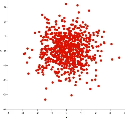
An example of a simple plot is a scatter chart, which plots a set of x-y pairs of numbers as points on a grid. These charts utilize the javafx.scene.chart.XYChart.Data and javafx.scene.chart.XYChart.Series classes. The Data class is a container that holds any dimension of mixed types of data, and the Series class contains an ObservableList of Data instances. There are factory methods in the
public class BasicScatterChart extends Application {
Figure 1-1. Scatter plot example
The ScatterChart class can readily be replaced with LineChart, AreaChart, or BubbleChart in the preceding example.
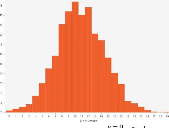
Bar charts
As an x-y chart, the bar chart utilizes the Data and Series classes. In this case, however, the only difference is that the x-axis must be a string type (as opposed to a numeric type) and utilizes the CategoryAxis class instead of the NumberAxis class. The y-axis remains as a NumberAxis.
Typically, the categories in a bar chart are something like days of the week or market segments. Note that the BarChart class takes a String, Number pair of types inside the diamonds. These are useful for making histograms, and we show one in Chapter 3:
public class BasicBarChart extends Application {
public static voidmain(String[] args) { launch(args);
}
@Override
String[] xData = {"Mon", "Tues", "Wed", "Thurs", "Fri"};
Multiple series of any type of plot are easily implemented. In the case of the scatter plot example, you need only to create multiple Series instances:
Seriesseries1 = new Series();
Seriesseries2 = new Series();
Seriesseries3 = new Series();
The series are then added in all at once using the addAll() method instead of the add() method:
scatterChart.getData().addAll(series1, series2, series3);
The resultant plot will show the points superimposed in various colors with a legend denoting their label name. The same holds true for line, area, bar, and bubble charts. An interesting feature here is the StackedAreaChart and StackedBarChart classes, which operate the same way as their respective AreaChart and BarChart superclasses, except that the data are stacked one above the other so they do not overlap visually.
charts of one type. However, we will demonstrate some workarounds later in this chapter.
Basic formatting
There are useful options for making your plot look really professional. The first place to cleanup might be the axes. Often the minor ticks are overkill. We can also set the plot range with minimum and maximum values:
At some point, it might be easier to keep the plotting mechanics simple and include all the style directives in a CSS file. The default CSS for JavaFX8 is called Modena and will be implemented if you don’t change the style options. You can create your own CSS and include it in the scene with this:
scene.getStylesheets().add("chart.css");
The default path is in the src/main/resources directory of your Java package.
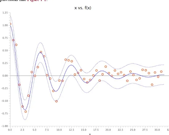
Plotting Mixed Chart Types
Often we want to display multiple plot types in one graphic—for example, when you want to display the data points as an x-y scatter plot and then overlay a line plot of the best fitted model. Perhaps you will also want to include two more lines to represent the boundary of the model, probably one, two, or three multiples of the standard deviation σ, or the confidence interval 1.96 × σ. Currently, JavaFX does not allow multiple plots of the different types to be displayed simultaneously on the same scene. There is a workaround, however! We can use a LineChart class to plot multiple series of LineChart instances and then use CSS to style one of the lines to show only points, one to only show a solid line, and two to show only a dashed line. Here is the CSS:
-fx-stroke: blue; -fx-stroke-width: 1;
-fx-stroke-dash-array: 1 4 1 4; }
/*.default-color0.chart-line-symbol { -fx-background-color: white, green; }*/
.default-color1.chart-line-symbol {
-fx-background-color: transparent, transparent; }
.default-color2.chart-line-symbol {
-fx-background-color: transparent, transparent; }
.default-color3.chart-line-symbol {
-fx-background-color: transparent, transparent; }
The plot looks like Figure 1-2.
Saving a Plot to a File
You will undoubtedly have an occasion to save a plot to a file. Perhaps you will be sending the plot off in an email or including it in a presentation. With a mixture of standard Java classes and JavaFX classes, you can easily save plots to any number of formats. With CSS, you can even style your plots to have publication-quality graphics. Indeed, the figures in this chapter (and the rest of the book) were prepared this way.
Each chart type subclasses the abstract class Chart, which inherits the method snapshot() from the Node class. Chart.snapshot() returns a WritableImage. There is one catch that must be addressed: in the time it takes the scene to render the data on the chart, the image will be saved to a file without the actual data on the plot. It is critical to turn off animation via Chart.setAnimated(false) someplace after the chart is instantiated and before data is added to the chart with Chart.getData.add() or its
equivalent:
/* do this right after the chart is instantiated */
scatterChart.setAnimated(false); ...
/* render the image */
stage.show(); ...
/* save the chart to a file AFTER the stage is rendered */
WritableImageimage = scatterChart.snapshot(new SnapshotParameters(), null);
Filefile = new File("chart.png");
ImageIO.write(SwingFXUtils.fromFXImage(image, null), "png", file);
Chapter 2. Linear Algebra
Now that we have spent a whole chapter acquiring data in some format or another, we will most likely end up viewing the data (in our minds) in the form of spreadsheet. It is natural to envision the names of each column going across from left to right (age, address, ID number, etc.), with each row representing a unique record or data point. Much of data science comes down to this exact
formulation. What we are seeking to find is a relationship between any number of columns of interest (which we will call variables) and any number of columns that indicate a measurable outcome
(which we will call responses).
Typically, we use the letter to denote the variables, and for the responses. Likewise, the responses can be designated by a matrix Y that has a number of columns and must have the same number of rows as X does. Note that in many cases, there is only one dimension of response variable such that . However, it helps to generalize linear algebra problems to arbitrary dimensions.
In general, the main idea behind linear algebra is to find a relationship between X and Y. The
simplest of these is to ask whether we can multiply X by a new matrix of yet-to-be-determined values
W, such that the result is exactly (or nearly) equal to Y. An example of XW = Y looks like this:
Keep in mind that as the equation is drawn, the sizes of the matrices look similar. This can be misleading, because in most cases the number of data points is large, perhaps in the millions or billions, while the number of columns for the respective X and Y matrices is usually much smaller (from tens to hundreds). You will then take notice that regardless of the size of (e.g.,
100,000), the size of the W matrix is independent of ; its size is (e.g., 10 × 10). And this is the heart of linear algebra: that we can explain the contents of extremely large data structures such as
X and Y by using a much more compact data structure W. The rules of linear algebra enable us to express any particular value of Y in terms of a row of X and column of W. For example the value of
is written out as follows:
those presented in Chapters 4 and 5, will rely heavily on the use of linear algebra.
Building Vectors and Matrices
Despite any formal definitions, a vector is just a one-dimensional array of a defined length. Many examples may come to mind. You might have an array of integers representing the counts per day of a web metric. Maybe you have a large number of “features” in an array that will be used for input into a machine-learning routine. Or perhaps you are keeping track of geometric coordinates such as x and y, and you might create an array for each pair [x,y]. While we can argue the philosophical meaning of what a vector is (i.e., an element of vector space with magnitude and direction), as long as you are consistent in how you define your vectors throughout the problem you are solving, then all the mathematical formulations will work beautifully, without any concern for the topic of study. In general, a vector x has the following form, comprising n components:
Likewise, a matrix A is just a two-dimensional array with m rows and n columns:
WARNING
We use bold lowercase letters to represent vectors and use bold uppercase letters to represent matrices. Note that the vector x can also be represented as a column of the matrix X.
In practice, vectors and matrices are useful to data scientists. A common example is a dataset in which (feature) vectors are stacked on top of each other, and usually the number of rows m is much larger than the number of columns n. In essence, this type of data structure is really a list of vectors, but putting them in matrix form enables efficient calculation of all sorts of linear algebra quantities. Another type of matrix encountered in data science is one in which the components represent a relationship between the variables, such as a covariance or correlation matrix.
Array Storage
The Apache Commons Math library offers several options for creating vectors and matrices of real numbers with the respective RealVector and RealMatrix classes. Three of the most useful constructor types allocate an empty instance of known dimension, create an instance from an array of values, and create an instance by deep copying an existing instance, respectively. To instantiate an empty, n -dimensional vector of type RealVector, use the ArrayRealVector class with an integer size:
intsize = 3;
RealVectorvector = new ArrayRealVector(size);
If you already have an array of values, a vector can be created with that array as a constructor argument:
double[] data = {1.0, 2.2, 4.5};
RealVectorvector = new ArrayRealVector(data);
RealVectorvector = new ArrayRealVector(realVector);
To set a default value for all elements of a vector, include that value in the constructor along with the size:
intsize = 3;
double defaultValue = 1.0;
RealVectorvector = new ArrayRealVector(size, defaultValue);
A similar set of constructors follows for instantiating matrices, an empty matrix of known dimensions is instantiated with the following:
introwDimension = 10;
intcolDimension = 20;
RealMatrixmatrix = new Array2DRowRealMatrix(rowDimension, colDimension);
Or if you already have a two-dimensional array of doubles, you can pass it to the constructor:
double[][] data = {{1.0, 2.2, 3.3}, {2.2, 6.2, 6.3}, {3.3, 6.3, 5.1}};
RealMatrixmatrix = new Array2DRowRealMatrix(data);
Although there is no method for setting the entire matrix to a default value (as there is with a vector), instantiating a new matrix sets all elements to zero, so we can easily add a value to each element afterward:
introwDimension = 10;
intcolDimension = 20;
double defaultValue = 1.0;
RealMatrixmatrix = new Array2DRowRealMatrix(rowDimension, colDimension);
matrix.scalarAdd(defaultValue);
Making a deep copy of a matrix may be performed via the RealMatrix.copy() method:
/* deep copy contents of matrix */
RealMatrixanotherMatrix = matrix.copy();
Block Storage
For large matrices with dimensions greater than 50, it is recommended to use block storage with the BlockRealMatrix class. Block storage is an alternative to the two-dimensional array storage
discussed in the previous section. In this case, a large matrix is subdivided into smaller blocks of data that are easier to cache and therefore easier to operate on. To allocate space for a matrix, use the following constructor:
Or if you already have the data in a 2D array, use this constructor:
double[][] data = ;
RealMatrixblockMatrix = new BlockRealMatrix(data);
Map Storage
When a large vector or matrix is almost entirely zeros, it is termed sparse. Because it is not efficient to store all those zeros, only the positions and values of the nonzero elements are stored. Behind the scenes, this is easily achieved by storing the values in a HashMap. To create a sparse vector of known dimension, use the following:
intdim = 10000;
RealVectorsparseVector = new OpenMapRealVector(dim);
And to create a sparse matrix, just add another dimension:
introws = 10000;
intcols = 10000;
RealMatrixsparseMatrix = new OpenMapRealMatrix(rows, cols);
Accessing Elements
Regardless of the type of storage backing the vector or matrix, the methods for assigning values and later retrieving them are equivalent.
CAUTION
Although the linear algebra theory presented in this book uses an index starting at 1, Java uses a 0-based index system. Keep this in mind as you translate algorithms from theory to code and in particular, when setting and getting values.
Setting and getting values uses the setEntry(int index, double value) and getEntry(int index) methods:
/* set the first value of v */
vector.setEntry(0, 1.2) /* and get it */
double val = vector.getEntry(0);
To set all the values for a vector, use the set(double value) method:
/* zero the vector */
vector.set(0);
retrieve all the values of an existing vector as an array of doubles, use the toArray() method:
double[] vals = vector.toArray();
Similar setting and getting is provided for matrices, regardless of storage. Use the setEntry(int row, int column, double value) and getEntry(int row, int column) methods:
/* set first row, 3 column to 3.14 */
matrix.setEntry(0, 2, 3.14); /* and get it */
double val = matrix.getEntry(0, 2);
Unlike the vector classes, there is no set() method to set all the values of a matrix to one value. As long as the matrix has all entries set to 0, as is the case for a newly constructed matrix, you can set all the entries to one value by adding a constant with code like this:
/* for an existing new matrix */
matrix.scalarAdd(defaultValue);
Just as with sparse vectors, setting all the values to 0 for each i,j pair of a sparse matrix is not useful. To get all the values of a matrix in the form of an array of doubles, use the getData() method:
double[][] matrixData = matrix.getData();
Working with Submatrices
We often need to work with only a specific part of a matrix or want to include a smaller matrix in a larger one. The RealMatrix class contains several useful methods for dealing with these common cases. For an existing matrix, there are two ways to create a submatrix from it. The first method selects a rectangular region from the source matrix and uses those entries to create a new matrix. The selected rectangular region is defined by the point of origin, the upper-left corner of the source
matrix, and the lower-right corner defining the area that should be included. It is invoked as
RealMatrix.getSubMatrix(int startRow, int endRow, int startColumn, int endColumn) and returns a RealMatrix object with dimensions and values determined by the selection. Note that the endRow and endColumn values are inclusive.
double[][] data = {{1,2,3},{4,5,6},{7,8,9}};
RealMatrixm = new Array2DRowRealMatrix(data);
intstartRow = 0;
intendRow = 1;
intstartColumn = 1;
intendColumn = 2;
We can also get specific rows and specific columns of a matrix. This is achieved by creating an array of integers designating the row and column indices we wish to keep. The method then takes both of these arrays as RealMatrix.getSubMatrix(int[] selectedRows, int[] selectedColumns). The three use cases are then as follows:
/* get selected rows and all columns */
int[] selectedRows = {0, 2};
int[] selectedCols = {0, 1, 2};
RealMatrixsubM = m.getSubMatrix(selectedRows, selectedColumns); // {{1,2,3},{7,8,9}}
/* get all rows and selected columns */
int[] selectedRows = {0, 1, 2};
int[] selectedCols = {0, 2};
RealMatrixsubM = m.getSubMatrix(selectedRows, selectedColumns); // {{1,3},{4,6},{7,9}}
/* get selected rows and selected columns */
int[] selectedRows = {0, 2};
int[] selectedCols = {1};
RealMatrixsubM = m.getSubMatrix(selectedRows, selectedColumns); // {{2},{8}}
We can also create a matrix in parts by setting the values of a submatrix. We do this by adding a double array of data to an existing matrix at the coordinates specified by row and column in RealMatrix.setSubMatrix(double[][] subMatrix, int row, int column):
double[][] newData = {{-3, -2}, {-1, 0}};
In learning algorithms, we often want to set all the values of a matrix (or vectors) to random numbers. We can choose the statistical distribution that implements the AbstractRealDistribution interface or just go with the easy constructor, which picks random numbers between –1 and 1. We can pass in an existing matrix or vector to fill in the values, or create new instances:
public class RandomizedMatrix {
private AbstractRealDistributiondistribution;
public RandomizedMatrix(AbstractRealDistributiondistribution, longseed) { this.distribution = distribution;
distribution.reseedRandomGenerator(seed); }